Download

1 / 43
430 likes | 591 Views
Stages in NN development. Specification. What is the problem we are trying to tackle? What is the performance required? Do you need an artificial neural network? i.e. will a simple statistical technique such as regression give acceptable performance?. Data.

E N D
Specification • What is the problem we are trying to tackle? • What is the performance required? • Do you need an artificial neural network? i.e. will a simple statistical technique such as regression give acceptable performance?
Data • Is there enough data available? If there is too little data we get ‘overfitting’. • As a good ‘guide’ to the amount of data required you will need 10 times as many data records as there are weights in the artificial neural network. e.g. given six inputs, say six hidden units and one output, then: (6 x 6) inputs to hidden layer and then (6 x 1) hidden feed to the output implies: 36 + 6 = 42 weights giving 42 x 10 = 420 data records.
Data • What form is the data in? Is it in a database? If so, extract to a flat file (or spreadsheet). • What is the quality of the data? • Are there missing values in the data? If so, do we throw that record away or do we impute (guess) at the missing value.
·A simple imputation (missing values): Name Age Sex Salary Mary 39 female 30 Fred 29 male 25 Tom 41 male ??? We can easily impute that Fred is a male. However it is difficult to impute a value for the salary for Tom. Sometimes can use statistics or artificial neural networks to impute this salary value. Nevertheless, we must sometimes balance this [Tom’s salary] against the number records are available. If we have many records we can throw this record away.
·Sometimes we have incorrect values: Name Age Occupation Peter 11 Schoolchild Amy 30 Employed Tom 90 Schoolchild Ella 223 Employed · Tom’s occupation can be correctly established as ‘retired’. However, is Ella 22 or 23? We must always check the data.
Performance evaluation • How are we going to evaluate the network?: % correctness? • RMS error - tells us how close we are getting to a real number. • True Positives, True Negatives, False Positives, False Negatives? - Get an idea of cost or profit/loss the network is making.
Construct the network Train the network Test the network on data it has not seen before (generalisation) Evaluate performance
Implementation • Then the best network is incorporated into an application e.g.: C/C++ function or VB code or whatever (may be invisible to the user).
Selecting data for neural networks • Data specification (and collection) - in which variables of interest are identified and collected. • Data inspection - in which data is examined and analysed. • These two steps are typically performed iteratively and in parallel with each other, and with the Data Pre-Processing phase (discussed later).
Issues • What information would we like to know? • What variables can be used to access the desired information? • Can other variables or relationships capture the same information indirectly?
Issues • Is a particular variable significant in a static context (i.e. is only the current value of that variable of interest) or is it important in a dynamic context (are historical trends of the variable important)? • Is the variable always used or is it used only in special cases? If so what are those cases? • Is this variable’s significance enhanced by additional variables (i.e. are combinations of variables important).
Issues • When a preliminary list of candidate variables has been compiled, the modeller must evaluate the viability of each of the variables. • This usually involves some kind of trade-off. • Certain variables may be important but not readily available.
Issues • For example, a modeller may discover that a certain type of test-marketing data is very useful in predicting future sales of a new product, but that such data is available for new products only half the time. • In such cases the modeller must compare the added benefits of using the variable with the hardship of obtaining it.
Significance • Several statistical methods are available for determining the significance of variables. Many of these are linear techniques, whereas neural networks are non-linear models. • However many linear techniques are easy to use, much easier than some of the non-linear techniques strictly applicable to neural networks. These linear techniques can be extremely useful in pointing out relationships in the data.
Correlation • Calculating the correlation coefficient for two variables can give an indication of the strength of the relationship between them – as it measures the degree to which two variables move together. Ranges from -1.0 to +1.0 • 0 = no correlation, 1.0 = high positive correlation (when x is high y is high), -1.0 indicating a high negative correlation (when x is high y is low). Correlation plots can depict these relationships graphically.
Correlation • Alternatively the correlation of two candidate input variables can be tested. • If the two variables are highly correlated it may be that we can combine them into a single input variable. • This can be useful if we wish to keep our network small.
Ordinary Least Squares (OLS) Regression Analysis: • This is a widely used statistical modelling technique that can be a useful tool for examining the linear significance of candidate variables. • OLS minimises the mean-squared errors of a linear function between variables. Several useful statistics are generated by OLS. • The t-statistic for each independent variable measures its significance in the model. • T-statistic values that are over 1.98 indicate that the variable is significant (for large samples)
Regression • Another statistic, the adjusted R2 (ranging from 0 to 1) indicates whether a given set of variables estimates the process being modelled for the available data set. • OLS regression is a powerful tool in itself and can often perform as well as a neural network on certain classes of problems (those which contain linear relationships). • In such cases it should be the technique used, as it is quick and simple.
Problems with tests of statistical significance and correlation. • Statistical significance and correlation do not always imply causality or predictive power. In other words, even if two variables grow or decay together, this does not necessarily imply that they are related in some causative way. • Correlation can take at least 3 forms:
x y (or y x) • Here the value of x will directly affect the value of y. For example, the number of hours that a particular machine is in operation (x) directly affects the number of widgets produced by that machine (y). • These kinds of relationships are ideal for modelling. • However, it should be noted that it may not be clear which variable causes the other.
x y (or y x) • Evidence of a causal relationship between two variables exists only if it can be shown that a change in one variable occurs only after a corresponding change in the first. • For example, if adding historical values of x to a model improves the models predictive power with respect to y, but adding y to a model does not increase the predictive power of the model with respect to x, then there is some evidence that x causes y.
z x and z y • In this case a third (possibly unknown) variable affects both x and y, even though no direct relationship exists between x and y. • For example, a produce distributor might notice that when the production of oranges (x) decreases, there is a corresponding decrease in the production of strawberries (y).
z x and z y • In this case the decrease in strawberry production is not caused by the decrease in orange production. Instead a third factor, such as the weather conditions during the growing season (z) affects them both.
x (not) y • This relationship can be the most misleading. • In this case two unrelated variables are (by coincidence) correlated. • Examples of this spurious correlation include the length of women’s hemlines and the output of the US economy, or the number of letters in the US president’s names and the sales of television sets in England.
x (not) y • Such spurious correlations occur when two series are generally increasing or decreasing over a particular sampling period. • If two seemingly unrelated variables are highly correlated, you may have discovered a new relationship. However it is more likely that the correlation is spurious and should not be relied on to predict a relationship in the future.
Data Inspection • After the data is identified and collected, it must be examined to identify any characteristics that may be unusual or indicative of more complex relationships. • This process is closely intertwined with data pre-processing (described later). The modeller will frequently use the techniques in this section to determine when pre-processing may be useful and what type of pre-processing might be appropriate.
Data Inspection • The first step in determining whether a particular variable needs pre-processing is to examine the distribution of the variable. • A useful tool for examining frequency distributions is the histogram, which slices up the range of possible variable values into equally-sized bins.
Histograms • When creating a histogram care must be taken that the endpoints and coarseness are chosen correctly. • The endpoints determine the maximum and minimum values to be plotted, and the coarseness determines the size and number of each bin. The second of the following figures shows a histogram that has these values chosen inappropriately.
Histograms • Often many histograms are created, and these help the modeller determine if there are outliers (see later) and whether the shape of the data has the correct distribution for a neural network.
Data distribution • Most modelling techniques (including neural networks) work best on normally distributed data. • However some data distributions are not normal, there are two measures which can be applied to the distributions to detect how far it is from a normal distribution:
Skewness • Skewness coefficient measures whether the distribution is symmetrical (is it shaped like a bell, a half bell or a dented bell). • In general, a skewness coefficient of -0.5 to 0.5 is considered to be a characteristic of a normally distributed variable. • Values greater than 0.5 indicate that the distribution is lopsided.
Kurtosis • Kurtosis measures the ‘fatness’ of the tails of a distribution. • Values of Kurtosis in the range -1.0 to 1.0 are generally thought to be characteristic of normal distributions.
Static versus dynamic context • In the following diagram, the two sample points give the same reading • Do you think we are helping the network by giving the same input value for both of these points?
Static versus dynamic context • No, the are obviously not the same, at one time the variable is climbing steeply, in the other falling steeply • So just giving a static value for that variable would be foolish • Instead give the value and rate of change (positive versus negative slope)
Outliers • Anomalous outliers can be one of the most disruptive influences on a quantitative model. • An outlier is an extreme data point that may have undue influence on a model. • Outliers are often (but not always) caused by erroneous data cases. • In the first figure a good approximation to relationship in the model is shown • In the second figure single outlier pulls this relationship off course so now fits data less well
Outliers • The outlier could have come from an incorrect data entry (such as someone accidentally typing 0 rather than 9 in a database) in which case we could just discard this data value. • However, if we did not know this we would want to investigate further. • The outlier could in fact be indicating important information. Perhaps the process is not linear.
Outliers • We can often spot outliers by examining histograms of the data. • Additionally some statistics related to OLS regression can be used to identify some types of outliers. • Remember that outliers are not always errors, these exceptions are sometimes the most useful indications of the underlying process. • If you cannot explain an anomaly, think twice before deleting it!
Summary • We have outlined the development cycle for a neural network application • We have discussed the importance of data selection