Motion in magnetic field: Classical Mechanics

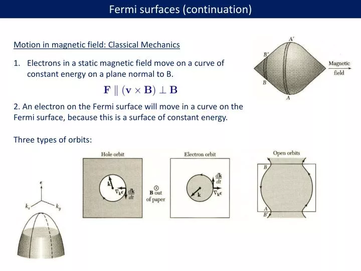
1. Fermi surfaces(continuation) Motion in magnetic field: Classical Mechanics Electrons in a static magnetic field move on a curve of constant energy on a plane normal to B. 2. An electron on the Fermi surface will move in a curve on the Fermi surface, because this is a surface of constant energy. Three types of orbits:

2. Vacant orbitals near the top of an otherwise filled band give rise to hole-like orbits Reduced band scheme Periodic band scheme Periodic band scheme Reduced band scheme Constant energy surface in the Brillouin zone of a simple cubic lattice

3. Fermi surfaces: Experimental Methods Powerful experimental methods have been developed for the determination of Fermi surfaces. The methods include magnetoresistance, anomalous skin effect, cyclotron resonance, magneto-acoustic geometric effects, the Shubnikov-de Haas effect, and the de Haas-van Alphen effect. Further information on the momentum distribution is given by positron annihilation. Following Kittel, we consider here the de Haas-van Alphen effect as the simplest one. Quantization of electron motion in magnetic field Following the semiclassical approach of Onsager and Lifshitz, we assume that the orbits in a magnetic field are quantized by the Bohr-Sommerfeldrelation where n is an integer and γis a phase correction that for free electrons has the value 1/2. In magnetic field, the current operator acquires an additional contribution (-e/c)A where A is the vector-potential of magnetic field. In SI system the factor 1/c is omitted.

4. According to equation of motion of a charge in magnetic field Then the first part of the path integral is where Φis the magnetic flux contained within the orbit in real space. We have used the geometrical result that The second path integral is:

5. Then we conclude that the orbit of an electron is quantized in such a way that the flux through it is In the de Haas-van Alphen effect discussed below we need the area of the orbit in wave vector space. Form the relation we know that a line element dr in the plane normal to Bis related to dkas so that the area Snin k space is related to the area Anof the orbit in r space by Therefore,

6. According to quantum mechanics, the wave function is smeared around classical trajectory over a distance of the order of the quantum length lM.

7. In Fermi surface experiments we may be interested in the increment ΔB for which two successive orbits, n and n + 1, have the same area in k space on the Fermi surface. The areas are equal when We have the important result that equal increments of 1/B reproduce similar orbits –this periodicity in 1/B is a striking feature of the magneto-oscillatory effects in metals at low temperatures: resistivity, susceptibility, heat capacity. De Haas-van Alphen Effect The de Haas-van Alphen effect is the oscillation of the magnetic moment of a metal as a function of the static magnetic field intensity. The effect can be observed in pure specimens at low temperatures in strong magnetic fields: we do not want the quantization of the electron orbits to be blurred by collisions, and we do not want the population oscillations to be averaged out by thermal population of adjacent orbits.

8. When we increase the field to B2 the total electron energy is increased, because the uppermost electrons have their energy raised. The field has a value B1such that the total energy of the electrons is the same as in the absence of a magnetic field: as many electrons have their energy raised as lowered by the orbital quantization in the magnetic field B1. For field B3the energy is again equal to that for the field B = O. The total energy is a minimum at points such as B1, B3, ... , and a maximum near points such as B2, B4, .

9. Let us discuss the case of absolute zero and concentrate on the plane perpendicular to B. The area between successive orbits in k-space is The area in k space occupied by a single orbital is (2π/L)2, neglecting spin, for a square specimen of side L. Therefore, the number of free electron orbitals that coalesce in a single magnetic level is Such a magnetic level is called a Landau level.

10. The dependence of the Fermi level on B is dramatic. For a system of N electrons at absolute zero the Landau levels are entirely filled up to a magnetic quantum number we identify by s, where s is a positive integer. Orbitalsat the next higher level s + 1 will be partly filled to the extent needed to accommodate the electrons. The Fermi level will lie in the Landau level s + 1 if there are electrons in this level; as the magnetic field is increased the electrons move to lower levels. When s + 1 is vacated, the Fermi level moves down abruptly to the next lower level s. The electron transfer to lower Landau levels can occur because their degeneracy D increases as B is increased. As B is increased there occur values of B at which the quantum number of the uppermost filled level decreases abruptly by unity. At the critical magnetic fields labeled Bs, no level is partly occupied at absolute zero, so that The number of filled levels times the degeneracy at B, must equal the number of electrons N.

11. (a) The heavy line gives the number of particles in levels which are completely occupied in a magnetic field B, for a two-dimensional system with N = 50 and ρ= 0.50. The shaded area gives the number of particles in levels partially occupied. The value of s denotes the quantum number of the highest level which is completely filled. Thus at B = 40 we have s = 2; the levels n = 1 and2 are filled and there are 10 particles in the level n = 3. At B = 50 the level n = 3 is empty. (b) The periodicity in 1/B is evident when the same points are plotted against1/B.

12. To show the periodicity of the energy as B is varied, we use the result that the energy of the Landau level of magnetic quantum number n is is the cyclotron frequency. The result for En follows from the analogy between the cyclotron resonance orbits and the simple harmonic oscillator, but now we have found it convenient to start counting at n = 1 instead of at n = O. The total energy of the electrons in levels that are fully occupied is The total energy of the electrons in the partly occupied level s + 1 is The total energy versus 1/B is shown in the next slide

13. The upper curve is the total electronic energy versus 1/B. The shaded region in the figure gives the contribution to the energy from levels that are only partly filled. The units are taken such that

14. The magnetic moment μof a system at absolute zero is given by The moment here is an oscillatory function of 1/B. This oscillatory magnetic moment of the Fermi gas at low temperatures is the de Haas-van Alphen effect. The oscillations occur at equal intervals of 1/B such that where S is the extremal area (see below) of the Fermi surface normal to the direction of B. From measurements of , we deduce the corresponding extremal areas S; thereby much can be inferred about the shape and size of the Fermi surface,

15. ExtremalOrbits One point in the interpretation of the dHvA effect is subtle. For a Fermi surface of general shape the sections at different values of kBwill have different periods. Here kBis the component of k along the direction of the magnetic field. The response will be the sum of contributions from all sections or all orbits. But the dominant response of the system comes from orbits whose periods are stationary with respect to small changes in kB. Such orbits are called extremal orbits.

16. Fermi Surface of Copper The Fermi surface of copper is distinctly non-spherical: eight necks make contact with the hexagonal faces of the first Brillouinzone of the fcc lattice. The electron concentration in a monovalent metal with an fcc structure is n = 4/a3 ; there are four electrons in a cube of volume a3. The radius of a free electron Fermi sphere is The shortest distance across the Brillouin zone (the distance between hexagonal faces) is , somewhat larger than the diameter of the free electron sphere. The sphere does not touch the zone boundary, but we know that the presence of a zone boundary tends to lower the band energy near the boundary. Thus it is plausible that the Fermi surface should neck out to meet the closest (hexagonal) faces of the zone

17. Dog's bone orbit of an electron on the Fermi surface of copper or gold in a magnetic field. This orbit is classified as hole-like because the energy increases toward the interior of the orbit.