Download
1 / 23
230 likes | 235 Views
Learn about option pricing models, put-call parity, upper and lower bounds, early exercise of American options, and using options as hedging tools.

E N D
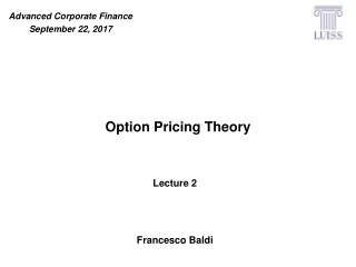
WEMBA 2000 Real Options 37 Option Pricing Models: Theoretical Justification For all possible values of the underlying asset at expiration: (i) Calculate the option payoff at that price (for a call: max[0, S-K]) (ii) Multiply the payoff by the probability of that outcome (iii) Discount the probability-weighted payoff at the riskless rate of interest (iv) Add together all discounted probability-weighted payoffs Example 106 c = 6 prob = 1/8 104 102 c=2 prob = 3/8 102 100 100 98 98 c=0 prob = 3/8 96 94 c=0 prob = 1/8 Note: error on handouts call value = (6 * 1/8 + 2 * 3/8) / (1.02)3 = 1.41
WEMBA 2000 Real Options 38 The Lognormal Distribution of Asset Returns Option pricing models assume that asset returns are distributed lognormally If asset prices are normally distributed, then returns are lognormally distributed (mathematical relationship) Empirically this has been shown to be the case over the long-run Useful characteristics of lognormal distribution: (a) returns cannot be negative (logarithms are never negative) (b) volatility remains constant in percentage terms Frequency of returns returns
WEMBA 2000 Real Options 39 Valuation of Options: Put-Call Parity We construct two portfolios and show they always have the same payoffs, hence they must cost the same amount. Portfolio 1: Buy 1 share of the stock today for price S0 and borrow an amount PV(K) = K e-rT How much will this portfolio be worth at time T ? Cashflow Cashflow Position Time = 0 Time = T Buy Stock -S0 ST Borrow PV(K) -K Net: Portfolio 1PV(K) - S0 ST - K Portfolio payoff at time T S Payoff from stock net payoff K ST Payoff from borrowing Payoff from borrowing -K
WEMBA 2000 Real Options 40 Valuation of Options: Put-Call Parity Portfolio 2: Buy 1 call option and sell 1 put option with the same maturity date T and the same strike price K. How much will this portfolio be worth at time T ? Cashflow Cashflow: Time = T Position Time = 0ST < K ST > K Buy Call - c 0 ST - K Sell Put p - (K - ST ) 0 Net: Portfolio 2p - c ST - K ST - K Portfolio payoff at time T Payoff on long call net payoff K ST Payoff on short put -K
WEMBA 2000 Real Options 41 Valuation of Options: Put-Call Parity Payoff from Portfolio 1 and Portfolio 2 is the same, regardless of level of ST , hence cost of both portfolios (cashflows at time T = 0 ) must be the same. Hence: S0 - PV(K) = c - pPut-Call Parity Rearranging: c = p + S0 - PV(K) (1) Put-Call parity: a worked example Stock is selling for $100. A call option with strike price $90 and maturity 3 months has a price of $12. A put option with strike price $90 and maturity 3 months has a price of $2. The risk-free rate is 5%. Question: Is there an arbitrage? Test Put-Call parity: Right-hand side of (1):p + S0 - PV(K) = 2 + 100 - 90 e -0.05*0.25 = 13.12 Left-hand side of (1): c = 12 13.12 ! Market Price of c is too low relative to the other three. Buy the call, and Sell the "replicating portfolio".
WEMBA 2000 Real Options 42 Valuation of Options: Upper and Lower bounds Upper Bounds: c Sp Ke -rT Today Value Time = T Position ST < K ST > K Sell Call c 0 -ST + K Buy Stock -S ST ST Net: c - S 0 ST 0 K 0 Today Value Time = T Position ST < K ST > K Sell put p ST - K 0 lend money -Ke-T K K Net: p - Ke-T 0 ST 0 K 0 Lower Bounds c > S - K e-rT p > K e-rT - S
WEMBA 2000 Real Options 43 Early Exercise of American Options Never optimal to exercise an American call (on a non-dividend paying stock) early S = 40 K = 30 T = 1 month (a)If you plan to hold the stock beyond expiration then don't exercise early (i) Earn 1 month interest on $30 (ii) Purchase the stock at expiration if it is still in-the-money (iii) If by chance it isn't in the money, you have saved yourself K-ST (b) If you plan to exercise and sell the stock immediately You will earn S - K by exercising the option, however…. … you should sell the option for c instead Q: How do you know c > S - K ? A: See lower bound on previous slide: c > S - K e-rT => c > S - K Hence camer = ceuroon non-dividend-paying stocks
WEMBA 2000 Real Options 44 Options as Hedging Tools Example 1: Portfolio Insurance Value Time = T Position ST < K ST > K Own Portfolio ST ST Buy Put (K - ST ) 0 Net: K ST Payoff on portfolio Portfolio payoff at time T Payoff on put net payoff K ST
WEMBA 2000 Real Options 45 Options as Hedging Tools Example 2: Currency Hedging--A worked example Polythene Providers Inc. has a global business supplying polythene and other synthetic products worldwide. The company's Treasurer, Pamela Mann, has just been informed that Polythene Providers Inc. may need to purchase supplies from the UK in 2 months for £2 million, and is concerned that the value of the pound may appreciate against the dollar in the interim period. So she purchases 2 million calls on Sterling with a strike of 1.6 $/£ (today's exchange rate level), expiring in two months. The call costs $10,800. If $/£ appreciates above 1.6, Mann can purchase £2 million at the strike of 1.6 for a cost of $3.2 mill. Suppose $/£ is 1.75 in two months. Without the call, Mann would have to pay 2*1.75 = $3.5 million With the call, she pays 2*1.6 = $3.2 million, plus $0.01 for the call: total = $3.21 million The call has saved 3.5 - 3.21 = $290,000 If $/£ depreciates, Mann will let the call expire worthless and purchase £2 million at the market rate. Suppose $/£ is 1.45 in two months. Mann pays 2*1.45 = $2.9 million plus $0.01 for the call: total = $2.91 million.
WEMBA 2000 Real Options 46 Project Evaluation: NPV vs. Real Option Valuation • An electricity generator has the opportunity to build a new power project. • Net cash flows are $100MM in the first year of operation. • Net cash flows in the second year of operation depend upon whether an entrepreneurial link is built to bypass a transmission “bottleneck”. • If the link goes ahead, demand for power from the new plant will be low and net cash flow will be $80 mm. • If the link does not go ahead, demand for power from the new plant will be high and net cash flow will be $125 mm. • Similar uncertainty surrounds Year 3 net cash flows. • Cash flows beyond Year 3 are perpetual.
WEMBA 2000 Real Options 47 Electricity Generator Case ... 156 0.5 125 0.5 0.5 ... 100 100 0.5 0.5 80 0.5 ... 64 Expected Net Cash Flow ... 100 103 105 ... 0 1 2 3
WEMBA 2000 Real Options 48 Electricity Generator Case Case 2 Case 1 • Now or never. • Cost to build is 1,000. • NPV=1,044 - 1,000 = 44. • Positive NPV. • Accept the project. • Now or never. • Cost to build is 1,100. • NPV=1,044 - 1,100 = -56. • Negative NPV. • Reject the project. Case 3 • Option to delay for one year. • During this one-year delay, the generator learns whether or not the new entrepreneurial link will proceed. • Based on this additional information, a “smarter” decision can be made. Case 3a: Cost to build is 1,100. Case 3b: Cost to build is 1,000
WEMBA 2000 Real Options 49 Electricity Generator Case ... 156 0.5 “up” state 125 0.5 ... 100 0.5 “down” state 80 0.5 ... 64 Expected Net Cash Flow in “up” state PV = 1,277 ... 125 128 Expected Net Cash Flow in “down” state PV = 818 ... 80 82 ... 0 1 2 3
WEMBA 2000 Real Options 50 Electricity Generator Case Case 3 Case 3a • Cost to build is 1,100. • proceed if “up state” NPV=1277-1100=177 • reject if “down state” NPV=0. • Expected NPV today is: • Compare with NPV without 1yr delay: NPV without delay = - 56 Difference: 136 Case 3b • Cost to build is 1,000. • proceed if “up state” NPV=1277-1000=277 • reject if “down state” NPV=0. • Expected NPV today is: • Compare with NPV without 1 yr delay: NPV without delay = 44 Difference: 82
... 156 Yearly Cash Flows 125 ... 100 100 80 One-time Liquidation Value 800 WEMBA 2000 Real Options 51 Electricity Generator Case Case 4 • Plant can be abandoned at any time for 800. Cost of building plant is 1000. • This option will be exercised whenever the PV of future cash flows falls below 800. • This only happens at the lowest node, where perpetual cash flows are 64. • When the abandonment option is incorporated, the NPV of building the project now is +77. • The NPV of waiting for one year is +126. • It is still optimal to delay for one year in this case, although the incremental value of delaying has decreased. • The value of the option to delay is lower if it is easy to exit a bad investment.
WEMBA 2000 Real Options 52 Electricity Generator Case: Conclusions • The option to delay can be valuable, even if the project has positive NPV if started immediately. • The value of these options is ignored by standard DCF techniques. • Proper analysis of these options is needed not just for project valuation, but also for project timing.
WEMBA 2000 Real Options 53 Case Study: Rigby Oil Rigby Oil owns the drilling rights for a small oil field in the North Sea. A drilling platform has been constructed, but extraction has not yet commenced. Rigby owns the drilling rights for the next five years. We have the following information: The current spot price of oil is $28 per barrel The annualized standard deviation of percentage changes in the price of oil is 40% p.a. The 3 month government bond rate is 6.00% p.a. and the 10yr government bond rate is 6.5% The estimated oil reserve in Rigby's oil field is 1.2 million barrels Extraction can proceed at the rate of 100,000 barrels per month The forward market for oil is highly liquid; hence oil can be sold forward at fair value (which implies that, for the purposes of the option model, you can sell all the oil that you extract at the spot price as of the day you begin extraction). The existing drilling platform uses out-of-date technology resulting in extraction costs of $25/barrel Before extraction can commence, startup costs of $6 million will be required to prepare the drilling equipment for operation A competitor, McKensey Oil, has offered Rigby $8 million for the drilling rights in their entirety.
WEMBA 2000 Real Options 54 Case Study: Rigby Oil (2) Traditional NPV analysis: Cashflows from extraction: - 6 + (28 - 25) * 1.2 = -$2.4 million reject Cashflow from selling the lease: = $8 million accept? Option-Adjusted Present Value analysis: S = K = T = r = = BS call value: Option cost: Option-adjusted PV =
WEMBA 2000 Real Options 55 Case Study: Rigby Oil (2) Traditional NPV analysis: Cashflows from extraction: - 6 + (28 - 25) * 1.2 = -$2.4 million reject Cashflow from selling the lease: = $8 million accept? Option-Adjusted Present Value analysis: S = K = T = r = = BS call value: Option cost: Option-adjusted PV = 33.6 ($28/barrel for 1.2 MM barrels) 30 ($25 extraction costs per barrel over 1.2 MM barrels) 4 (you need to start drilling in 4 years if you are to complete extraction within 5 years) 6.25% (we need a 4-year rate. Try interpolating between the 3 month and 10 year rates, and test sensitivity of results to this assumption) 40% 15 6 9 Keep the Option!
WEMBA 2000 Real Options 56 Case Study: Rigby Oil (3) Option to wait Suppose the decision facing Rigby Oil were changed as follows: startup costs were only $3 million no option to sell the lease to the competitor NPV analysis: - 3 + (28 - 25) *1.2 = $0.6 million Accept? No! Should not exercise early! If you want to exercise the call and immediately sell the underlying asset (the oil), what should you do instead? Sell the option! There may not be a buyer for the lease at a fair market price (this is not a liquid financial option) How do we earn the fair market value of the option if there isn't a buyer? [HINT: remember the "replicating portfolio" method of valuing options]
(a) Near perfect tracking (b) Imperfect tracking WEMBA 2000 Real Options 57 Caveats for using Financial Options Models on Real Options Binomial pricing methods require the potential to buy or sell the underlying asset to create replicating or riskless portfolio. [Note: it is not necessary to actually buy/sell the underlying asset. Options are priced relative to the price of the underlying security--relying on accurate valuation of that security by the financial markets]. What if the underlying asset when the company is not publicly traded? Can we use alternative, traded assets to proxy for the “real” underlying asset? If so: Tracking risk: How closely do they mimic the performance of the real asset? Transactions costs: It may be costly to create and dynamically update a replicating portfolio of assets
WEMBA 2000 Real Options 58 Tracking Portfolio Risks Basis Risk: Northern Farms expands into organic bread baking, and enters into a supply contract on organic flour from midwestern flour mill. Northern Farms hedges the flour price risk with wheat options since flour is not a traded commodity. Massive floods in the midwest take out rail transportation lines. Cost of organic flour increases substantially, while wheat prices are relatively unaffected. Leakage: Owning a physical commodity may have benefits or costs that do not accrue to owners of derivatives on the commodity. If you own aluminum and there is an unexpected price increase because of shortages, you can earn a convenience yield by feeding some of your supply into the market. Alternatively, increased storage costs may work against you if there is a short-term glut on a commodity. (The resultant price drop is reflected in the derivative value, but the increased storage costs are not). Private Risk: Sun King Technology is considering a radical new design for Sun workstation chips. They have two concerns: (1) whether the chip will be developed in time and on budget, and (2) whether the market demand for Sun workstations will be buoyant when they bring the new chip to market. (2) is market risk, and can be hedged (e.g. by purchasing options on other Sun workstation stocks, or other assets closely allied with the market for computer hardware). However, (1) is private risk, and cannot be hedged.
WEMBA 2000 Real Options 59 Using Financial Options Models on Real Options When can we use options models in the "real" world? When the project outcomes closely mimic the price performance of a liquid, traded security whose returns are distributed lognormally, so that the "replicating portfolio" option pricing theory is justified Why do we use financial options models in the "real" world? Options theory provides insight into the uncertain and changing nature of capital pricing decisions, and offers a better method for evaluating projects in the face of uncertainty than traditional "static" models (such as NPV) What are the principal differences between the options approach and the NPV approach? Options are more valuable when projects are risky (i.e. cash flows are volatile) Option theory enables us to use a single, riskless discount rate throughout