Download
1 / 37
370 likes | 396 Views
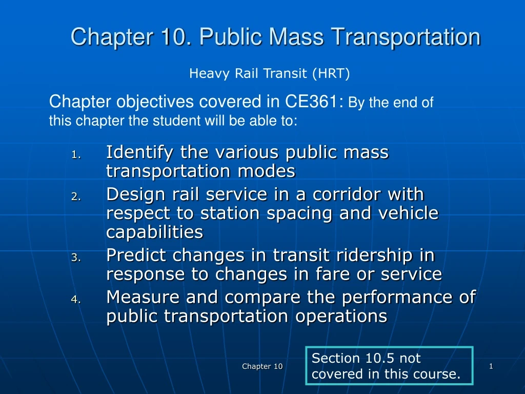
Heavy Rail Transit (HRT). Chapter objectives covered in CE361: By the end of this chapter the student will be able to:. Chapter 10. Public Mass Transportation. Identify the various public mass transportation modes

E N D
Heavy Rail Transit (HRT) Chapter objectives covered in CE361: By the end of this chapter the student will be able to: Chapter 10. Public Mass Transportation Identify the various public mass transportation modes Design rail service in a corridor with respect to station spacing and vehicle capabilities Predict changes in transit ridership in response to changes in fare or service Measure and compare the performance of public transportation operations Section 10.5 not covered in this course. Chapter 10
10.1 Transit Modes • Objectives of 10.1 • Name different transit modes • Explain the niches of different transit modes By the end of this section, the student will be able to... Chapter 10
10.1 Transit Modes Public Mass Transportation several meanings. Here we will focus on that subset of public mass transit that has the following characteristics: • A common carrier • Fixed route and fixed schedule • The area served is limited to an urban area or a rural area (Intercity service is called “intercity mass transportation”) NYCMTA NJ Hudson-Bergen LRT Others: Paratransit Long Island RR/Jamaica Sta. JFK Airport Chapter 10 Staten Island Ferry
Portland’s Max Light Rail Transit (LRT) Portland Airport Bike racks Portland Downtown Chapter 10
France’s TGV Heavy Rail Transit (HRT) Chapter 10
Japan’s Shinkansen Heavy Rail Transit (HRT) Linear motor train: 2027 operation begins (planned) Chapter 10
Shanghai’s Maglev Chapter 10
Japan’s Maglev (test) Test speed reached 500 kph (313 mph) recently. (Tokyo – Nagoya: Planned operation begins in 2027) Japan, France, China, Germany: Their governments invest in public transit. How about the US government? Chapter 10
Public transport system classified by routing and scheduling types Scheduling (frequency of service) Chapter 10 Routing (degree of coverage and access)
Prof. VucanVuchic’s classification BRT TRAX Front Runner Chapter 10
Driverless RRT example Seoul, KoreaDriverless subway line (70 kph) Gangnam Station – do you remember that song? Chapter 10
Visiting public transit agencies in Germany Berlin Dresden Cologne Bamberg Heidelberg Ulm Karlsruhe Munich Augsberg Chapter 10
Public Transit: Keys to Success • Intermodality (transfer from a mode to another mode is simple and easy) • Convenient ticket pricing and vending • Multiline coverage of major areas of a city • Service to passengers Munich Chapter 10
Public Transit: Keys to Success (continued) Cologne Chapter 10
Modern Airport-like RR Station Berlin Central Chapter 10
10.2 Designing Rail Transit Line • Objectives of 10.2 • Explain the trade-offs available for dealing with accessibility and mobility • Determine transit vehicle travel regimes in terms of travel distance and time By the end of this section, the student will be able to... Chapter 10
10.2 Designing Rail Transit Line (with respect to station spacing and vehicle capabilities) 10.2.1 Transit Vehicle Travel Analysis Goal of providing service: (a) increase access to as many riders as it can, and at the same time (b) Minimize the time it takes to carry passengers from their origins to their destinations. The trade-off to achieve these two conflicting goals becomes: • Increase the number of stops along a route • Reduce the number of stops (Increase travel speed) Strategy B: B1. Determine the best distance between transit stops on a route to make the best use of the performance characteristics of the transit vehicles assigned to the route B2. Determine the best performance characteristics for transit vehicles assigned to a particular route, given a specified spacing between transit stops on that route Chapter 10
Trax vs. Frontrunner (Trade off example) Chapter 10
FrontRunner in Utah County Chapter 10
10.2.2 Transit Vehicle Regimes The goal: Maximize the average operating speed along the route (& at the same time save energy as much as possible).Acceleration, deceleration, and maximum speed are the three key vehicle performance characteristics. Diagram of Five Transit Travel Regimes: 2 3 1 Acceleration & Deceleration: 3-4 mph/s (4.42–5.9 ft/s2) Jerk (Rate of change of accel or decel rate): 1.12-2.68 m/s3 (3.6–8.79 ft/s3) 5 4 Station Standing Time Chapter 10 Travel Regime Diagram
Equations for Transit Vehicle Travel Regimes Examine these equations carefully. Eq. 10.12 (shown below) does not contain the constant speed regime. S = sa + sc + sb,c Chapter 10
Examples 10.1 – 10.3 • We will walk through these examples. Chapter 10
10.3 Predicting Transit Ridership Changes • Objectives of 10.3 • Define elasticity. • Tell the difference between “elastic” and “inelastic” demand. • Determine elasticity values, such as fare elasticity of transit, service elasticity, etc. By the end of this section, the student will be able to... Chapter 10
10.3 Predicting Transit Ridership Changes 10.3.2 Transit Elasticity with respect to Fare • Elasticity = (% change in quantity of service purchased)/(% change in price of service) Pay attention to the sign of the shrinkage ratio Shrinkage Ratio = Elasticity • The value of the shrinkage ratio is one way of measuring the demand elasticity of transit ridership with respect to fare. • When the sign of the shrinkage ratio is negative, the quantity of service purchased decreases. The number of passenger will decrease. • A typical value for public transit is – 0.33 (meaning 1% increase in fare will cause 0.33% decrease in ridership). Chapter 10
Mythaca Bus Company case If the value of the shrinkage factor was -0.33, ridership would have decreased down to: Chapter 10
Recent study on fare elasticity • Fare Elasticity-Bus Services Average (all hours all cities) -0.40 (apparently greater than -0.33 mentioned in the textbook). Chapter 10 Source: APTA website
Fare elasticity • Fare elasticity = Elasticity of transit ridership with respect to fare. Before: $0.75 x 10,000 = $7,500 After: $1.00 x8,750 = $8,750 • If revenue will increase, despite a fare increase, the demand is “inelastic,” which is the case above. Another way of saying this is if the shrinkage factor (elasticity, ε) is -1 < ε < 0, ridership is “inelastic” to fare increase. • If revenues will decrease as the fare increases, the demand is “elastic.” Or, if elasticity, ε, is less than -1, ridership is “elastic” to fare increase. This concept is very important when transit agencies consider fare hikes. In the case above, MBC ridership is fare elastic or fare inelastic? Chapter 10
Example 10.4 Predicting transit revenue changes by fare category using demand elasticity Chapter 10
Example 10.4 (continued) Chapter 10 Which category is fare elastic or inelastic?
10.3.3 Transit Elasticity with Respect to Service • Elasticity of transit ridership with respect to service • Typical headway elasticities are -0.37 during peak hours and -0.46 in the off-peak. • How do we express “service” by headway or frequency Chapter 10 We will walk through Examples 10.5 & 10.6.
10.4 Performance Measures in Public Transportation • Objectives of 10.4 • Evaluate a transit system’s operation using performance measures. • Distinguish longitudinal analysis from peer group analysis. By the end of this section, the student will be able to... Chapter 10
10.4.1 Transit performance measures Need to have a set of performance measures and their criteria to compare the performance level of a transit system with the performance levels of similar systems (of a peer group). • Effectiveness (do the right thing) vs. efficiency (doing something well) For example, ridership is an effectiveness measure, while cost per mile is an efficiency measure. Chapter 10
Transit Performance Measures - samples Accessibility related PMs: • Average travel time • Average trip length • Percent of population within x miles of employment • Percent of population that can reach services by transit, bicycle, or walking • Percent of transit dependent population • Percent of transfers between modes to be under x minutes and n feet • Transfer distance at passenger facility • Percent of workforce that can reach worksite by transit within one hour and with no more than two transfers • Percent of population within access to transit service • Percent of urban and rural areas with direct access to passenger rail and bus service • Access time to passenger facility • Route miles of transit service • Route spacing • Percent of total transit trip time spent out of vehicle • Existence of information services and ticketing • Availability of park and ride Chapter 10
Mobility related PMs • Percent on-time performance • Percent of scheduled departures that do not leave within a specified time limit • Travel time contour • Minute variation in trip time • Fluctuations in traffic volumes • Average transfer time/delay • Dwell time at intermodal facilities • Proportion of persons delayed • In-vehicle travel time • Frequency of service • Average wait time to board transit • Number of public transportation trips Chapter 10
Performance measures - samples See Table 10.4 • TVM (total vehicle miles) • Revenue vehicle miles • Ridership • Cost/mi • Cost/trip • Fare box recovery ratio • % Labor See Example 10.7 Chapter 10
UTA Performance Measures UTA performance report 2014 Chapter 10
What’s longitudinal analysis? (P. 10.25) • It’s an analysis method that compares the performance measures of then and now. Used when peers are not available. • Must compare performance measures taken under similar conditions. (Before and after analyses must be done in a similar environment, meaning, if the before data were taken in January, after data may need to be taken January of the following year. Read Example 10.8. It is straight forward. Chapter 10