Download

1 / 38
380 likes | 386 Views
Oscillator models of the Solar Cycle and the Waldmeier-effect. Melinda Nagy MSc Astronomy Department of Astronomy, ELTE Supervisor Dr. Kristóf Petrovay Department of Astronomy, ELTE. 6 th Workshop of Young Researchers in Astronomy and Astrophysics, 2012. Budapest. Our objectives were….

E N D
Oscillator models of the Solar Cycle and the Waldmeier-effect Melinda Nagy MSc Astronomy Department of Astronomy, ELTE Supervisor Dr. Kristóf PetrovayDepartment of Astronomy, ELTE Oscillator models of the Solar Cycle and the Waldmeier-effect 6th Workshop of Young Researchers in Astronomy and Astrophysics, 2012. Budapest
Our objectives were… By varying the parameters of the van der Pol oscillator: • To reproduce the Waldmeier-effect • To approximate other known properties of the Solar Cycle To extend the model to van der Pol-Duffing oscillator and vary the parameters together Oscillator models of the Solar Cycle and the Waldmeier-effect
Modern maximum Maunder minimum Dalton minimum The Solar Cycle • Sunspot Number, introduced by Wolf (1859): asymmetric, cyclic behaviour • From minimum to maximum: 3-4 years • From maximum to minimum: 7-8 years • The degree of the asymmetry correlates to the amplitude of the cycle Oscillator models of the Solar Cycle and the Waldmeier-effect
The Solar Cycle • The degree of the asymmetry correlates to the amplitude of the cycle • first formulated by Waldmeier (1935) as an inverse correlation between rise time and the cycle maximum • the effect is clearer if we use the rise rate instead of rise time • Correlation coefficient in the case of rise rate (left panel) and decay rate (right panel): no significant link between this and the amplitude of the cycle r = 0.22 r = 0.83 Cameron & Schüssler(2008) Oscillator models of the Solar Cycle and the Waldmeier-effect
The Solar Cycle Usoskin (2007): sunspot number reconstruction by 14C data for 11000 years. The distribution can be characterized with Gaussian curve (=30, =31) Oscillator models of the Solar Cycle and the Waldmeier-effect
Oscillator model of the Solar Cycle To produce grand minima, they also used van der Pol -Duffing oscillator, Lopes & Passos (2011). They kept constant the parameters (, ,λ), and was increased temporary – it caused grand minima like behaviour: Lopes & Passos (2008) fitted van der Pol-Duffing oscillator on each magnetic cycle – λ was neglected. The main value of these fitted parameters: Oscillator models of the Solar Cycle and the Waldmeier-effect
Oscillator model of the Solar Cycle To produce grand minima, they also used van der Pol -Duffing oscillator, Lopes & Passos (2011). They kept constant the parameters (, ,λ), and was increased temporary – it caused grand minima like behaviour: Lopes & Passos (2008) fitted van der Pol-Duffing oscillator on each magnetic cycle – λ was neglected. The main value of these fitted parameters: Oscillator models of the Solar Cycle and the Waldmeier-effect
The method of our study • The behaviour of the van der Pol oscillator was analyzed by making its parameters time dependent : • , dumping parameter and , nonlinearity • The requirements were: • Waldmeier-effect: correlation coefficient > 0.8 • the absolute value ofcorrelation between decay rate and the amplitude < 0.5 • the deviation of the cycle length and that of the amplitude should be more than 10% • Amplitude-time functions were calculated for an interval of 2000 years • We used Lopes & Passos (2008) fitted parameters as constants Oscillator models of the Solar Cycle and the Waldmeier-effect
The method of our study • The behaviour of the van der Pol oscillator was analyzed by making its parameters time dependent : • , dumping parameter and , nonlinearity • The requirements were: • Waldmeier-effect: correlation coefficient > 0.8 • the absolute value ofcorrelation between decay rate and the amplitude < 0.5 • the deviation of the cycle length and that of the amplitude should be more than 10% • Amplitude-time functions were calculated for an interval of 2000 years • We used Lopes & Passos (2008) fitted parameters as constants Oscillator models of the Solar Cycle and the Waldmeier-effect
The method of our study • The behaviour of the van der Pol oscillator was analyzed by making its parameters time dependent : • , dumping parameter and , nonlinearity • The requirements were: • Waldmeier-effect: correlation coefficient > 0.8 • the absolute value ofcorrelation between decay rate and the amplitude < 0.5 • the deviation of the cycle length and that of the amplitude should be more than 10% • Amplitude-time functions were calculated for an interval of 2000 years • We used Lopes & Passos (2008) fitted parameters as constants Oscillator models of the Solar Cycle and the Waldmeier-effect
The method of our study • The behaviour of the van der Pol oscillator was analyzed by making its parameters time dependent : • , dumping parameter and , nonlinearity • The requirements were: • Waldmeier-effect: correlation coefficient > 0.8 • the absolute value ofcorrelation between decay rate and the amplitude < 0.5 • the deviation of the cycle length and that of the amplitude should be more than 10% • Amplitude-time functions were calculated for an interval of 2000 years • We used Lopes & Passos (2008) fitted parameters as constants Oscillator models of the Solar Cycle and the Waldmeier-effect
The method of our study We used the equation of the Van der Pol oscillator and we varied its parameters: and separately, using different methods. In the case of : • delta-correlated noise, K is the relaxation parameter • constant value for a defined time interval (correlation time) We used these methods in two different way to create (t) and (t), in addition, we restricted the values to keep the oscillator stable. • additive noise • multiplicative noise Oscillator models of the Solar Cycle and the Waldmeier-effect
The method of our study We used the equation of the Van der Pol oscillator and we varied its parameters: and separately, using different methods. In the case of : • delta-correlated noise, K is the relaxation parameter • constant value for a defined time interval (correlation time) We used these methods in two different way to create (t) and (t), in addition, we restricted the values to keep the oscillator stable. • additive noise • multiplicative noise Oscillator models of the Solar Cycle and the Waldmeier-effect
The method of our study We used the equation of the Van der Pol oscillator and we varied its parameters: and separately, using different methods. In the case of : • delta-correlated noise, K is the relaxation parameter • constant value for a defined time interval (correlation time) We used these methods in two different way to create (t) and (t), in addition, we restricted the values to keep the oscillator stable. • additive noise • multiplicative noise Oscillator models of the Solar Cycle and the Waldmeier-effect
The method of our study We used the equation of the Van der Pol oscillator and we varied its parameters: and separately, using different methods. In the case of : • delta-correlated noise, K is the relaxation parameter • constant value for a defined time interval (correlation time) We used these methods in two different way to create (t) and (t), in addition, we restricted the values to keep the oscillator stable. • additive noise • multiplicative noise Oscillator models of the Solar Cycle and the Waldmeier-effect
The method of our study We used the equation of the Van der Pol oscillator and we varied its parameters: and separately, using different methods. In the case of : • delta-correlated noise, K is the relaxation parameter • constant value for a defined time interval (correlation time) We used these methods in two different way to create (t) and (t), in addition, we restricted the values to keep the oscillator stable. • additive noise • multiplicative noise Oscillator models of the Solar Cycle and the Waldmeier-effect
Constant variation for a defined correlation time:With multiplicative‘submethod’: Results I. A 300 years long part from the calculated 2000 years: Oscillator models of the Solar Cycle and the Waldmeier-effect
Solar Cycle r = 0.83 Cameron & Schüssler(2008) Results I. van der Pol oscillator Waldmeier-effect Oscillator models of the Solar Cycle and the Waldmeier-effect
Oscillator models of the Solar Cycle and the Waldmeier-effect
Oscillator models of the Solar Cycle and the Waldmeier-effect
Oscillator models of the Solar Cycle and the Waldmeier-effect
Results II. A 300 years long part from the calculated 2000 years: Oscillator models of the Solar Cycle and the Waldmeier-effect
Results II. 11 000 years long simulation: • Parameters of the fitted Gaussian curve: • Mean value: 52.96 • Standard deviation: 24.24 • In the case of the Sun: • Usoskin (2007), =30, =31 Oscillator models of the Solar Cycle and the Waldmeier-effect
Summary • We tested the nonlinear, van der Pol(-Duffing) oscillator as a basic model by varying its parameters stochastically. • The main goal was to reproduce the Waldmeier effect, and approximate other statistically features of the Solar Cycle. • Conclusions: • the model reproduces the Waldmeier effect and our other requirements, even if the varied parameter is only • it can show grand minima, but to keep the proper cycle length and shape, the other parameters also should be varied beside • the amplitude distribution of the cycles can show excess at low and high levels, too, compared to a Gaussian fit Oscillator models of the Solar Cycle and the Waldmeier-effect
Summary • We tested the nonlinear, van der Pol(-Duffing) oscillator as a basic model by varying its parameters stochastically. • The main goal was to reproduce the Waldmeier effect, and approximate other statistically features of the Solar Cycle. • Conclusions: • the model reproduces the Waldmeier effect and our other requirements, even if the varied parameter is only • it can show grand minima, but to keep the proper cycle length and shape, the other parameters also should be varied beside • the amplitude distribution of the cycles can show excess at low and high levels, too, compared to a Gaussian fit Oscillator models of the Solar Cycle and the Waldmeier-effect
Summary • We tested the nonlinear, van der Pol(-Duffing) oscillator as a basic model by varying its parameters stochastically. • The main goal was to reproduce the Waldmeier effect, and approximate other statistically features of the Solar Cycle. • Conclusions: • the model reproduces the Waldmeier effect and our other requirements, even if the varied parameter is only • it can show grand minima, but to keep the proper cycle length and shape, the other parameters also should be varied beside • the amplitude distribution of the cycles can show excess at low and high levels, too, compared to a Gaussian fit Oscillator models of the Solar Cycle and the Waldmeier-effect
Summary • We tested the nonlinear, van der Pol(-Duffing) oscillator as a basic model by varying its parameters stochastically. • The main goal was to reproduce the Waldmeier effect, and approximate other statistically features of the Solar Cycle. • Conclusions: • the model reproduces the Waldmeier effect and our other requirements, even if the varied parameter is only • it can show grand minima, but to keep the proper cycle length and shape, the other parameters also should be varied beside • the amplitude distribution of the cycles can show excess at low and high levels, too, compared to a Gaussian fit Oscillator models of the Solar Cycle and the Waldmeier-effect
Summary • We tested the nonlinear, van der Pol(-Duffing) oscillator as a basic model by varying its parameters stochastically. • The main goal was to reproduce the Waldmeier effect, and approximate other statistically features of the Solar Cycle. • Conclusions: • the model reproduces the Waldmeier effect and our other requirements, even if the varied parameter is only • it can show grand minima, but to keep the proper cycle length and shape, the other parameters also should be varied beside • the amplitude distribution of the cycles can show excess at low and high levels, too, compared to a Gaussian fit Thank you for your attention! Oscillator models of the Solar Cycle and the Waldmeier-effect
Summary • We tested the nonlinear, van der Pol(-Duffing) oscillator as a basic model by varying its parameters stochastically. • The main goal was to reproduce the Waldmeier effect, and approximate other statistically features of the Solar Cycle. • Conclusions: • the model reproduces the Waldmeier effect and our other requirements, even if the varied parameter is only • it can show grand minima, but to keep the proper cycle length and shape, the other parameters also should be varied beside • the amplitude distribution of the cycles can show excess at low and high levels, too, compared to a Gaussian fit Thank you for your attention! Oscillator models of the Solar Cycle and the Waldmeier-effect
Oscillator models of the Solar Cycle and the Waldmeier-effect
11 000 years long simulation: • Parameters of the fitted Gaussian curve: • mean value: 34.25 • standard deviation: 33.06 the average cycle length: 12.68 yr the longest cycle: 19.58 yr Oscillator models of the Solar Cycle and the Waldmeier-effect
A 1000 years long part from the calculated 11000 years: Oscillator models of the Solar Cycle and the Waldmeier-effect
A 400 years long part from the calculated 2000 years: Constant variation for a defined correlation time:With additive‘submethod’: Oscillator models of the Solar Cycle and the Waldmeier-effect
40 ~30 years long Oscillator models of the Solar Cycle and the Waldmeier-effect
The Waldmeier effect is shown All the required statistical parameter is shown Correlation between the rise rate and the amplitude of the cycles • van der Pol-Duffing oscillator, x1.5(t), varied parameters: , and λ • is defined as delta-correlated noise, with multiplicative submethod • connection is defined between the parameters Oscillator models of the Solar Cycle and the Waldmeier-effect
The Waldmeier effect is shown All the required statistical parameter is shown Correlation between the rise rate and the amplitude of the cycles • van der Pol oscillator, x1.5(t) • varied parameter: • constant for the interval of the correlation time, used multiplicatively Oscillator models of the Solar Cycle and the Waldmeier-effect
Oscillator model of the Solar Cycle To produce grand minima, they also used van der Pol -Duffing oscillator, Lopes & Passos (2011). They kept constant the parameters (, ,λ), and was increased temporary – it caused grand minima like behaviour: Lopes & Passos (2008) fitted van der Pol-Duffing oscillator on each magnetic cycle – λ was neglected. The main value of these fitted parameters: Oscillator models of the Solar Cycle and the Waldmeier-effect
Oscillator models of the Solar Cycle and the Waldmeier-effect