Download
1 / 22
220 likes | 335 Views
CS 170: Computing for the Sciences and Mathematics. More Accurate Rate Estimation. Administrivia. Last time (in P265) Euler’s method for computation Today Better Methods Simulation / Automata HW #7 Due! HW #8 assigned. Euler’s method.

E N D
CS 170:Computing for the Sciences and Mathematics More Accurate Rate Estimation
Administrivia • Last time (in P265) • Euler’s method for computation • Today • Better Methods • Simulation / Automata • HW #7 Due! • HW #8 assigned
Euler’s method • Simplest simulation technique for solving differential equation • Intuitive • Some other methods faster and more accurate • Error on order of ∆t • Cut ∆t in half cut error by half
Euler’s Method • tn = t0 + n t • Pn = Pn-1 + f(tn-1, Pn-1) t
Runge-Kutta 2 method • Euler's Predictor-Corrector (EPC) Method • Better accuracy than Euler’s Method • Predict what the next point will be (with Euler) – then correct based on estimated slope.
Concept of method • Instead of slope of tangent line at (tn-1, Pn-1), want slope of chord • For ∆t = 8, want slope of chord between (0, P(0)) and (8, P(8))
Concept of method • Then, estimate for 2nd point is ? • (∆t, P(0) + slope_of_chord * ∆t) • (8, P(0) + slope_of_chord * 8)
Concept of method • Slope of chord ≈ average of slopes of tangents at P(0) and P(8)
EPC • How to find the slope of tangent at P(8) when we do not know P(8)? • Y = Euler’s estimate for P(8) • In this case Y = 100+ 100*(.1*8) = 180 • Use (8, 180) in derivative formula to obtain estimate of slope at t = 8 • In this case, f(8, 180) = 0.1(180) = 18 • Average of slope at 0 and estimate of slope at 8 is • 0.5(10 + 18) = 14 • Corrected estimate of P1 is 100 + 8(14) = 212
Runge-Kutta 2 Algorithm initialize simulationLength, population, growthRate, ∆t numIterations simulationLength / ∆t fori going from 1 to numIterations do the following: growth growthRate * population Y population + growth * ∆t t i*∆t population population+ 0.5*( growth + growthRate*Y) estimating next point (Euler) averaging two slopes
Error • With P(8) = 15.3193 and Euler estimate = 180, relative error = ? • |(180 - P(8))/P(8)| ≈ 19.1% • With EPC estimate = 212, relative error = ? • |(212 - P(8))/P(8)| ≈ 4.7% • Relative error of Euler's method is O(t)
EPC at time 100 t Estimated P Relative error • 1.0 2,168,841 0.015348 • 0.5 2,193,824 0.004005 • 0.25 2,200,396 0.001022 • Relative error of EPC method is on order of O((t)2)
Runge-Kutta 4 • If you want increased accuracy, you can expand your estimations out to further terms. • base each estimation on the Euler estimation of the previous point. • P1 = P0 + d1, d1 = rate*P0*Dt • P2 = P1 + d2, d2 = rate*P1*Dt • P3 = P2 + d3, d3 = rate*P2*Dt • d4 = rate*P3*Dt • P1 = (1/6)*(d1 + 2*d2 + 2*d3 + d4) • error: O(Dt4)
CS 170:Computing for the Sciences and Mathematics Simulation
Computer simulation • Having computer program imitate reality, in order to study situations and make decisions • Applications?
Use simulations if… • Not feasible to do actual experiments • Not controllable (Galaxies) • System does not exist • Engineering • Cost of actual experiments prohibitive • Money • Time • Danger • Want to test alternatives
Example: Cellular Automata • Structure • Grid of positions • Initial values • Rules to update at each timestep • often very simple New = Old + “Change” • This “Change” could entail a diff. EQ, a constant value, or some set of logical rules
Mr. von Neumann’s Neighborhood • Often in automata simulations, a cell’s “change” is dictated by the state of its neighborhood • Examples: • Presence of something in the neighborhood • temperature values, etc. of neighboring cells
Conway’s Game of Life • The Game of Life, also known simply as Life, is a cellular automaton devised by the British mathematician John Horton Conway in 1970. • The “game” takes place on a 2-D grid • Each cell’s value is determined by the values of an expanded neighborhood (including diagonals) from the previous time-step. • Initially, each cell is populated (1) or empty (0) • Because of Life's analogies with the rise, fall and alterations of a society of living organisms, it belongs to a growing class of what are called simulation games (games that resemble real life processes).
Conway’s Game of Life The Rules • For a space that is 'populated': • Each cell with one or zero neighbors dies (loneliness) • Each cell with four or more neighbors dies (overpopulation) • Each cell with two or three neighbors survives • For a space that is 'empty' or 'unpopulated‘ • Each cell with three neighbors becomes populated http://www.bitstorm.org/gameoflife/
HOMEWORK! • Homework 8 • READ “Seeing Around Corners” • http://www.theatlantic.com/magazine/archive/2002/04/seeing-around-corners/2471/ • Answer reflection questions – to be posted on class site • Due THURSDAY 11/4/2010 • Thursday’s Class in HERE (P265)