Download
1 / 44
440 likes | 608 Views
Chemical Modelling & Data Assimilation D. Fonteyn, S. Bonjean, S. Chabrillat, F. Daerden and Q. Errera Belgisch Instituut voor Ruimte – Aëronomie (Belgian Institute for Space Aeronomy) BIRA - IASB. >> OUTLINE. Introduction What is chemical data assimilation?

E N D
Chemical Modelling & Data Assimilation • D. Fonteyn, S. Bonjean, S. Chabrillat, F. Daerden and Q. Errera • Belgisch Instituut voor Ruimte – Aëronomie • (Belgian Institute for Space Aeronomy) • BIRA - IASB A NICE PLACE
>> OUTLINE • Introduction • What is chemical data assimilation? • Why do we need chemical data assimilation? • 4D –VAR chemical data assimilation system • Physical consistency, Self consistency, Independent observations • Added value • Inverse modelling: emission estimations A NICE PLACE
>> OUTLINE Belgian Assimilation System of Chemical Observations from Envisat (BASCOE) http://bascoe.oma.be IMAGES A NICE PLACE
>> Introduction • Focus on the Stratosphere: • Chemical processes are well understood: high level of confidence in modelling results. (?) • Mature remote sensing technology (UARS, ENVISAT, SAGE, CRISTA, POAM …) • If models are perfect, no data assimilation is needed A NICE PLACE
>>Introduction>> Overview chemistry • Gas phase chemistry • Chapman Cycle • O2 + h 2O • O2 + O + M O3 + M • O3 + O 2O2 • O3 + h O2 + O • Catalytic cycles • Hydrogen radicals (HOx) • OH + O H + O2 • H + O3 OH + O2 • Net: O + O3 2 O2 • OH + O H + O2 • H + O2 + M HO2+ M • HO2 + O OH + O2 • Net: O + O3 O2 • HO2+ O OH + O2 • OH + O3 HO2 + O2 • Net: O + O3 2 O2 • Hydrogen Source Gases: H2O, CH4 • Long term trends • HOx chemistry in the upper stratosphere and mesosphere A NICE PLACE
>>Introduction>> Overview chemistry • Nitrogen radicals (member of NOy) • NO2 + O NO + O2 • NO + O3 NO2 + O2 • Net: O + O3 2 O2 • Chlorine radicals (member of Cly) • ClO + O Cl + O2 • Cl + O3 ClO + O2 • Net: O + O3 2 O2 • Nitrogen Source Gas: N2O (and …) • Long term trends • NOy partitioning (in the lower stratosphere: aerosols ) • Chlorine Source Gases: Organic Chlorine • Long term trends • Cly partitioning (in the lower stratosphere: aerosols ) A NICE PLACE
>> Chemical data assimilation • Chemical data assimilation • Inert tracer assimilation • Tracer with parameterized chemistry assimilation • Multiple species with chemical interactions • • Necessity A NICE PLACE
>>Why chemical data assimilation>> Model shortcomings TOMS total ozone 28 August 2003 A NICE PLACE
>>Why chemical data assimilation>> Model shortcomings Free model total ozone 28 August 2003, 12 UTC A NICE PLACE
>>Why chemical data assimilation >> Model shortcomings HALOE CH4 monthly gridded zonal mean, August 2003 ppmv A NICE PLACE
>>Why chemical data assimilation >> Model shortcomings HALOE CH4 monthly gridded zonal mean, August 2003 Free Model Run co-located, isolines ppmv A NICE PLACE
>> Why chemical data assimilation >> Model shortcomings Problem: input dynamics, confirmed by mean age of air experiment A NICE PLACE
CH4 >> Why chemical data assimilation >> Model shortcomings • GEM STRATO (MSC) with BASCOE chemistry vs. BASCOE driven by ECMWF • 3 month free model run • Same initial conditions • Matching resolution • Identical chemistry • No Feedback A NICE PLACE
>> Why chemical data assimilation >> Model shortcomings BASCOE driven by GEM-STRATO vs BASCOE driven by ECMWF CH4 A NICE PLACE
>> Why chemical data assimilation >> Model shortcomings BASCOE driven by GEM-STRATO vs BASCOE driven by ECMWF Ozone A NICE PLACE
>> Why chemical data assimilation >> Model shortcomings BASCOE driven by GEM-STRATO vs BASCOE driven by ECMWF Total ozone A NICE PLACE
>> Why chemical data assimilation >> Model shortcomings • Model Shortcomings: • Effect of dynamical assimilation • Effect of different dynamical assimilation systems • Dynamics driven shortcomings • Chemical modelling shortcomings (not shown) A NICE PLACE
>> 4D – VAR 4D-var assimilation : find x(t0) minimizing J With the constraint x(t0): control variable n 5.6 106 xb: a priori state of the atmosphere ( background) yo(ti): observations, de dimension p 5 104 (-7 105) x(ti): model state H: observational operator M: model operator B: background error covariance matrix R: observational error covariance matrix A NICE PLACE
>> 4D – VAR >> BASCOE • Model (3D - Chemical Transport Model) • horizontal: 3°.75 x 3°.75 (96 x 49 pts); vertical: 37 pressure levels, surface → 0.1 hPa (subset of ECMWF hybrid levels, keeping stratospheric levs) • 57 chemical species (control variables), 200 reactions • 4 types of PSC particles (36 size bins): NOT assimilated • Eulerian, driven by ECMWF 6h analyses/forecast • advection by Lin & Rood (1996) with 30’ time step • Assimilation set-up • Adjoint of chemistry and transport • Assimilation time window: 24 hours • B diagonal; 20 % of first guess distribution (= univariate) • Quality check: 1st climatoligical behaviour; 2 nd first guess based QC • Observations • ESA Envisat MIPAS L2 products, Near Real Time (NRT) and Offline (OFL) • O3, H2O, N2O, CH4, HNO3, NO2 • Representativeness error: 8.5 % A NICE PLACE
4D – VAR >> BASCOE >> OFL number of observations A NICE PLACE
4D – VAR >> BASCOE >> Multi-variate nature • Multi variate nature • Diagonal B • (xa(t0)-xb(t0)) • Local noon and local midnight • August, 7, 2003 • Full: observed species • Striped: unobserved species A NICE PLACE
4D – VAR >> BASCOE >> Physical consistency August 5, 2003 35.8 hPa & obs within 1 km A NICE PLACE
4D – VAR >> BASCOE >> Physical consistency Tracer correlations: CH4 vs N2O (Aug 5) Tropical South polar MIPAS DATA Co-located FMR Co-located analysis = correlation Needs validation A NICE PLACE
4D – VAR >> BASCOE >> Self – consistency • OmF: • Observation – first guess • Normalized by R • = Gaussian distribution • OFL • NRT • FMR • OFL vs NRT • Consistency • Added value w.r.p FMR A NICE PLACE
4D – VAR >> BASCOE >> Self – consistency >> model improvement • NRT results: • Ozone @ 1 hPa underestimated • Analysis = free model • Model not constrained • O2 main source of O3 • O2 not a control variable • JO2 increased by 25 % • New free model • Better agreement A NICE PLACE
4D – VAR >> BASCOE >> Self – consistency Self – consistency 4D – VAR: E[Janalysis] = p/2 Time series Janalysis/p NRT OFL Monitoring capability A NICE PLACE
4D – VAR >> BASCOE >> Self – consistency >> monitoring Monitoring capability Daily mean MIPAS ozone, [-10,10] at 14 hPa Janalysis transients correlate with ozone daily mean transients A NICE PLACE
4D – VAR >> BASCOE >> Example • Illustrative example: • August 5, 2003 • Lat: -38.6° Lon: 83.3° • NRT vs OFL data • Quality check • Pre-check • OI qc • First guess • Analysis • At 1 hPa: methane rich tropical air, and tropical dry air A NICE PLACE
4D – VAR >> BASCOE >> Independent observations • Independent observations: • HALOE v19 • Periode: August 2003 • Individual profiles • Statistics CH4 H2O Individual profile OFL analysis HALOE Free Model run A NICE PLACE
4D – VAR >> BASCOE >> HALOE August 2003 (HALOE-BASCOE)/HALOE OFL analysis NRT analysis HALOE error O3 H2O CH4 A NICE PLACE
4D – VAR >> BASCOE >> HALOE August 2003 NOx Mean HALOE and BASCOE co-located profiles: OFL analysis NRT analysis HALOE Ozone model bias & 4D – VAR chemical coupling reduces Cly HCl A NICE PLACE
4D – VAR >> BASCOE >> Added value HALOE and BASCOE co-located gridded zonal monthly mean OFL analysis FMR HALOE OFL analyis vs Free Model (Schoeberl et al., JGR 2003) A NICE PLACE
4D – VAR >> BASCOE >> Added value TOMS total ozone 28 August 2003 A NICE PLACE
4D – VAR >> BASCOE >> Added value Analysis total ozone 28 August 2003, 12 UTC A NICE PLACE
4D – VAR >> BASCOE >> Added value >> Chemical forecasts The operational implementation with NRT MIPAS allows to produce chemical forecasts Examples with verification A NICE PLACE
4D – VAR >> BASCOE >> Added value Operational implementation A NICE PLACE
4D – VAR >> BASCOE >> Added value A NICE PLACE
4D – VAR >> BASCOE >> Conclusions • 4D –VAR chemical data assimilation system • Multi-variate nature of 4D – VAR • Benefit • Model bias sensitivity • Overall Consistency • Independent observations • Added value (non-exhaustive) • Monitoring • Bias detection • Correction for dispersive dynamics • Chemical forecasts • Potential related to efforts A NICE PLACE
>> Inverse modelling • Inverse modelling at BIRA – IASB • J. – F. Muller & J. Stavrakou • Belgisch Instituut voor Ruimte – Aëronomie • (Belgian Institute for Space Aeronomy) • BIRA - IASB A NICE PLACE
>> Inverse modelling Focus: Tropospheric reactive gases (ozone precursors CO, NOx, non-methane VOCs) A NICE PLACE
>> Inverse modelling J(f)=½Σi (Hi(f)-yi)TE-1(Hi(f)-yi)+ ½ (f-fB)TB-1(f-fB) Matrix of errors on the observations Matrix of errors on the emission parameters first guess value for the control parameters Model operator acting on the control variables observations A NICE PLACE
>> Inverse modelling • Find best values of emission parameters, i.e. minimize the cost function • Previous studies for reactive gases (CO, NOx, CH2O) inverted for a small number of emission parameters (big-region approach) • Most previous studies used a linearized CTM, (i.e. OH unchanged by emission updates) straightforward minimization of the cost (matrix inversion) • Non-linearity is best handled using the adjoint model technique (Muller & Stavrakou 2005) also used in 4D-Var assimilation • This technique allows also to perform grid-based inversions A NICE PLACE
>> Inverse modelling • Grid – based inversion • Observations used: CO columns from MOPITT (05/2000 – 04/2001) • Model used: IMAGES, 5°x5° (Müller and Stavrakou 2005) • Number of control parameters >> number of independent observations • need additional information : correlations between errors on a priori emissions, estimated based on country boundaries, ecosystem distribution, geographical distance A NICE PLACE
>> Inverse modelling A NICE PLACE