Download
1 / 67
670 likes | 756 Views
Neural Networks: A Statistical Pattern Recognition Perspective. Instructor: Tai-Yue (Jason) Wang Department of Industrial and Information Management Institute of Information Management. Statistical Framework.

E N D
Neural Networks: A Statistical Pattern Recognition Perspective Instructor: Tai-Yue (Jason) Wang Department of Industrial and Information Management Institute of Information Management
Statistical Framework • The natural framework for studying the design and capabilities of pattern classification machines is statistical • Nature of information available for decision making is probabilistic
Feedforward Neural Networks • Have a natural propensity for performing classification tasks • Solve the problem of recognition of patterns in the input space or pattern space • Pattern recognition: • Concerned with the problem of decision making based on complex patterns of information that are probabilistic in nature. • Network outputs can be shown to find proper interpretation of conventional statistical pattern recognition concepts.
Pattern Classification • Linearly separable pattern sets: • only the simplest ones • Iris data: classes overlap • Important issue: • Find an optimal placement of the discriminant function so as to minimize the number of misclassifications on the given data set, and simultaneously minimize the probability of misclassification on unseen patterns.
Notion of Prior • The prior probabilityP(Ck) of a pattern belonging to class Ck is measured by the fraction of patterns in that class assuming an infinite number of patterns in the training set. • Priors influence our decision to assign an unseen pattern to a class.
Assignment without Information • In the absence of all other information: • Experiment: • In a large sample of outcomes of a coin toss experiment the ratio of Heads to Tails is 60:40 • Is the coin biased? • Classify the next (unseen) outcome and minimize the probability of mis-classification • (Natural and safe) Answer: Choose Heads!
Introduce Observations • Can do much better with an observation… • Suppose we are allowed to make a single measurement of a feature x of each pattern of the data set. • x is assigned a set of discrete values {x1, x2, …, xd}
Joint and Conditional Probability • Joint probabilityP(Ck,xl) that xl belongs to Ck is the fraction of total patterns that have value xl while belonging to class Ck • Conditional probabilityP(xl|Ck) is the fraction of patterns that have value xl given only patterns from class Ck
Number of patterns with value xl in class Ck Total number of patterns Number of patterns in class Ck Joint Probability = Conditional Probability Class Prior
Posterior Probability: Bayes’ Theorem • Note: P(Ck, xl) = P(xl, Ck) • P(Ck, xl) is the posterior probability: probability that feature value xl belongs to class Ck • Bayes’ Theorem
Bayes’ Theorem and Classification • Bayes’ Theorem provides the key to classifier design: • Assign patternxlto classCKfor which the posterior is the highest! • Note therefore that all posteriors must sum to one • And
Bayes’ Theorem for Continuous Variables • Probabilities for discrete intervals of a feature measurement are then replaced by probability density functions p(x)
Two-class one dimensional Gaussian probability density function variance mean normalizing factor Gaussian Distributions Distribution Mean and Variance
Example of Gaussian Distribution • Two classes are assumed to be distributed about means 1.5 and 3 respectively, with equal variances 0.25.
Extension to n-dimensions • The probability density function expression extends to the following • Mean • Covariance matrix
Covariance Matrix and Mean • Covariance matrix • describes the shape and orientation of the distribution in space • Mean • describes the translation of the scatter from the origin
Probability Contours • Contours of the probability density function are loci of equal Mahalanobis distance
Classification Decisions withBayes’ Theorem • Key: Assign X to Class Ck such that or,
Placement of a Decision Boundary • Decision boundary separates the classes in question • Where do we place decision region boundaries such that the probability of misclassification is minimized?
Quantifying the Classification Error • Example: 1-dimension, 2 classes identified by regions R1, R2 • Perror = P(x R1, C2) + P(x R2, C1)
Quantifying the Classification Error • Place decision boundary such that • point x lies in R1 (decide C1) if p(x|C1)P(C1) > p(x|C2)P(C2) • point x lies in R2 (decide C2) if p(x|C2)P(C2) > p(x|C1)P(C1)
Optimal Placement of A Decision Boundary Bayesian Decision Boundary: The point where the unnormalized probability density functions crossover
An artificial neuron implements the discriminant function: Each of C neurons implements its own discriminant function for a C-class problem An arbitrary input vector X is assigned to class Ck if neuron k has the largest activation Probabilistic Interpretation of a Neuron Discriminant Function
Probabilistic Interpretation of a Neuron Discriminant Function • An optimal Bayes’ classification chooses the class with maximum posterior probability P(Cj|X) • Discriminant function yj = P(X|Cj) P(Cj) • yjnotation re-used for emphasis • Relative magnitudes are important: use any monotonic function of the probabilities to generate a new discriminant function
Probabilistic Interpretation of a Neuron Discriminant Function • Assume an n-dimensional density function • This yields, • Ignore the constant term, assume that all covariance matrices are the same:
Plotting a Bayesian Decision Boundary: 2-Class Example • Assume classes C1, C2, and discriminant functions of the form, • Combine the discriminants y(X) = y2(X) – Y1(X) • New rule: • Assign X to C2 if y(X) > 0; C1 otherwise
Plotting a Bayesian Decision Boundary: 2-Class Example • This boundary is elliptic • If K1 = K2 = K then the boundary becomes linear…
Cholesky Decomposition of Covariance Matrix K • Returns a matrix Q such that QTQ = K and Q is upper triangular
Interpreting Neuron Signals as Probabilities: Gaussian Data • Gaussian Distributed Data • 2-Class data,K2 = K1 = K • From Bayes’ Theorem, we have the posterior probability
Interpreting Neuron Signals as Probabilities: Gaussian Data • Consider Class 1 Sigmoidal neuron ?
Interpreting Neuron Signals as Probabilities: Gaussian Data • We substituted • or, Neuron activation !
Interpreting Neuron Signals as Probabilities • Bernoulli Distributed Data • Random variable xi takes values 0,1 • Bernoulli distribution • Extending this result to an n-dimensional vector of independent input variables
Interpreting Neuron Signals as Probabilities: Bernoulli Data • Bayesian discriminant Neuron activation
Interpreting Neuron Signals as Probabilities: Bernoulli Data • Consider the posterior probability for class C1 where
Interpreting Neuron Signals as Probabilities: Bernoulli Data
Multilayered Networks • The computational power of neural networks stems from their multilayered architecture • What kind of interpretation can the outputs of such networks be given? • Can we use some other (more appropriate) error function to train such networks? • If so, then with what consequences in network behaviour?
Likelihood • Assume a training data set T={Xk,Dk} drawn from a joint p.d.f. p(X,D) defined onnp • Joint probability or likelihood of T
Sum of Squares Error Function • Motivated by the concept of maximum likelihood • Context: neural network solving a classification or regression problem • Objective: maximize the likelihood function • Alternatively: minimize negative likelihood: Drop this constant
Error function is the negative sum of the log-probabilities of desired outputs conditioned on inputs A feedforward neural network provides a framework for modelling p(D|X) Sum of Squares Error Function
Normally Distributed Data • Decompose the p.d.f. into a product of individual density functions • Assume target data is Gaussian distributed • j is a Gaussian distributed noise term • gj(X) is an underlying deterministic function
From Likelihood to Sum Square Errors • Noise term has zero mean and s.d. • Neural network expected to provide a model of g(X) • Since f(X,W) is deterministic p(dj|X) = p(j)
From Likelihood to Sum Square Errors • Neglecting the constant terms yields
Interpreting Network Signal Vectors • Re-write the sum of squares error function • 1/Q provides averaging, permits replacement of the summations by integrals
Interpreting Network Signal Vectors • Algebra yields • Error is minimized when fj(X,W) = E[dj|X] for each j. • The error minimization procedure tends to drive the network map fj(X,W) towards the conditional average E[dj,X] of the desired outputs • At the error minimum, network map approximates the regression of d conditioned on X!