Download
1 / 16
160 likes | 211 Views
The Hardy-Weinberg Equilibrium Model: Two Examples. Place: New York State Population: 10,000,000 Character of the disease: caused by the recessive allele and the recessive homozygous genotype is 100% fatal. Alleles: T, t. Example #1 Tay -Sachs Disease.

E N D
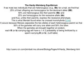
Place: New York State Population: 10,000,000 Character of the disease: caused by the recessive allele and the recessive homozygous genotype is 100% fatal. Alleles: T, t Example #1 Tay-Sachs Disease
TT Tt tt 9,697,700 300,000 2,300 Step #1 Divide the number of people in each genotype by the total population in order to determine the frequency of each genotype in the population. TT = 9,697,700/10,000,000 = .96977 Tt = 300,000/10,000,000 = .03 tt = 2,300/10,000,000 = .00023 These are your observed genotype frequencies.
Step #2 Calculate the allele frequencies. To calculate the frequency of the T allele, you have to count the number of T alleles in each genotype. Remember, everybody has two alleles. T = 2 x 9, 697,700 = 19,395,400 + 300,000 = 19,695,400 This has to be divided by the total number of alleles in the population = 20,000,000. 19,695,400/20,000,000 = .98477 = p
The same for the t allele: t = 2 x 2300 = 4,600 + 300,000 = 304,600 304,600 / 20,000,000 = .01523 = q Both allele frequencies should add up to 1. If not, then there has been a mistake in the math somewhere.
Step number 3: use the allele frequencies in the Hardy-Weinberg Equilibrium model. This will give you genotype frequencies that are in equilibrium. p2 + 2(pq) + q2=1 TT Tttt (.98477)2 + 2(.98477 x .01523) + (.01523)2= 1 .96977 .029996 .00023 These are the expected genotype frequencies. They do not represent the genotype frequencies of a real population.
Step #4: Compare the observed (real) genotype frequencies with the expected genotype frequencies (projection) to see if the observed genotype frequencies are in equilibrium. TT Tt tt observed: _ .96977 _.03 _ .00023 expected: .96977.029996 .00023 .0 .000004 0 Result: The original population is in equilibrium. There are no forces affecting this population.
Place: Nigeria. Population: 12,387. Character of the disease: Caused by the deleterious HbS allele. This allele is codominant with the HbA allele. Example #2: Sickle Cell Anemia
HbA HbA HbA HbS HbS HbS 9365 2993 29 Step #1 Calculate the observed genotype frequencies. 9365/12,387 2993/12,387 29/12,387 =.7560 =.2416 =.0023
Step #2: Calculate the allele frequencies. HbA = (2 x 9,365) + 2,993/(12,387x2) 21,723/24,774 = .8768 = p HbS = (2 x 29) + 2,993/(12,387 x 2) 3051/24,774 = .1232 = q
Step #3: Place the values for p and q into the Hardy-Weinberg Equilibrium model to calculate the expected genotype frequencies. (.8768)2 + 2(.8768 x .1232) + (.1232)2 = 1 .7688 + .2160 + .0152 = 1
Step #4: Compare the observed genotype frequencies with the expected genotype frequencies to determine whether or not the observed population is in equilibrium. Observed: _ .7560 _.2416 _.0023 Expected: .7688 .2160 .0152 .0128* .0256 .0129* Conclusion: The genotypes of the observed population are in disequilibrium as there is a significant difference between the observed and expected values. * Only absolute differences are relevant.
Since the population is in disequilibrium, looking at how the genotypes of the population are affected is warranted. First we want to measure the survival efficiency of the three genotypes. To do this, we divide the observed genotype frequencies by the expected genotype frequencies. Distinguishing the Impact of selection
HbAHbA HbAHbS HbSHbS Observed: .7560 .2416 .0023 Expected: .7688 .2160 .0152 Survival efficiency: .9833 1.185 .1513 If a survival efficiency statistic is higher than 1, then the people who have this genotype are doing rather well in the given environment. The reverse is true for values lower than 1. The heterozygotes are doing the best.
We can gain some additional insights into selection by adjudging the fitness of the genotypes relative to each other. We accomplish this by making the most successful genotype the standard of fitness, and then by dividing all three genotypes by this value. Relative Fitness
.9833 1.185 .1513 1.185 1.185 1.185 =.83 = 1 =.13 The homozygote genotype HbAHbA has 83% of the fitness of the heterozygote genotype, while the homozygote HbSHbS genotype has 13% of the fitness of the heterozygote. Selection is acting against both homozygotes. HbA HbA HbAHbS HbSHbS