Download
1 / 22
240 likes | 347 Views
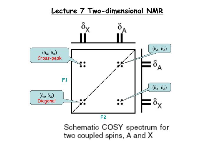
Lecture 7 Two-dimensional NMR. ( A , A ). ( A , X ) Cross-peak. F1. ( X , A ). ( x , X ) Diagonal. F2. Interpretation of peaks in 2D spectrum. Need mixing time to transfer magnetization to see cross peaks !. Allows interaction to take place. 1 H excitation.

E N D
Lecture 7 Two-dimensional NMR (A, A) (A, X) Cross-peak F1 (X, A) (x, X) Diagonal F2
Interpretation of peaks in 2D spectrum Need mixing time to transfer magnetization to see cross peaks !
Allows interaction to take place 1H excitation General scheme: To keep track of 1H magnetization (Signal not recorded) Signal contains info due to the previous three steps t1 = 0 Experiment: Get a series of FIDs with incremental t1 by a time . Thus, for an expt with n traces t1 For the traces will be 0, , 2, 3, 4 ----- (n-1), respectively. We will obtain a series of n 1D FID of S1(t1, t2). Fourier transform w.r.t. t2 will get a series of n 1D spectra S2(t1, 2). Further transform w.r.t. t1 will get a 2D spectrum of S3(1,2). Spectral width in the t1 (F1) dimension will be SW = 1/ FT F2 = 1 FT t1 = F2 = 2 t1 = 2 F2 = 1 t1 = 3 F2 = 3 t1 = 4 F2 = 4 t1 = 5 F2 = N t1 = n
Review on product operator formalism: • 1. At thermal equilibrium: I = Iz • 2. Effect of a pulse (Rotation): • exp(-iIa)(old operator)exp(iIa) = cos (Old operator) + sin (new operator) • 3. Evolution during t1 : • (free precession) (rotation w.r.t. Z-axis): = - Iy for 1tp = 90o Product operator for two spins: Cannot be treated by vector model Two pure spin states: I1x, I1y, I1z and I2x, I2y, I2z I1x and I2x are two absorption mode signals and I1y and I2y are two dispersion mode signals. These are all observables (Classical vectors)
Coupled two spins:Each spin splits into two spins Anti-phase magnetization:2I1xI2z, 2I1yI2z, 2I1zI2x, 2I1zI2y (Single quantum coherence) (Not observable) Double quantum coherence:2I1xI2x, 2I1xI2y, 2I1yI2x, 2I1yI2y(Not observable) Zero quantum coherence:I1zI2z (Not directly observable) Including an unit vector, E, there are a total of 16 product operators in a weakly-coupled two-spin system. Understand the operation of these 16 operators is essential to understand multi-dimensional NMR expts.
Example 1: Free precession of spin I1x of a coupled two-spin system: Hamiltonian: Hfree = 1I1z + 2I2z = cos1tI1x + sin1tI1y No effect Example 2: The evolution of 2I1xI2z under a 90o pulse about the y-axis applied to both spins: Hamiltonian: Hfree = 1I1y + 1I2y
Evolution under coupling: Hamiltonian: HJ= 2J12I1zI2z Causes inter-conversion of in-phase and anti-phase magnetization according to the Diagram, i.e. in-phase anti-phase and anti-phase in-phase according to the rules: Must have only one component in the X-Y plane !!!
Coherence order: Only single quantum coherences are observables • Single quantum coherences (p = ± 1): Ix, Iy, 2I1zI2y, I1yI2z, 2I1xI2z …. etc • Zero quantum coherence: Iz, I1z2z • Raising and lowering operators:I+ = ½(Ix + iIy); I- = 1/2 (Ix –i-Iy) • Coherence order of I+ is p = +1 and that of I- is p = -1 • Ix = ½(I+ + I-); Iy = 1/2i (I+ - I-)are both mixed states contain order p = +1 and p = -1 For the operator: 2I1xI2x we have: 2I1xI2x = 2x ½(I1+ + I1-) x ½(I2+ + I2-) = ½(I1+I2+ + I1-I2-) + ½(I1+I2- + I1-I2+) The double quantum part, ½(I1+I2+ + I1-I2-) can be rewritten as: Similar the zero quantum part can be rewritten as: ½(I1+I2- + I1-I2+) = ½ (2I1xI2x – 2I1yI2y) P = +2 P = -2 P = 0 P = 0 (Pure double quantum state) (Pure zero quantum state)
2D-NOESY of two spins w/ no J-coupling: • Consider two non-J-coupled spin system: • Before pulse:: Itotal = • Let us focus on spin 1 first: • 2. 90o pulse (Rotation): 3. t1 evolution: 4. Second 90o pulse: 5. Mixing time: Only term with Iz can transfer energy thru chemical exchange. Other terms will be ignored. This term is frequency labelled (Dep. on 1 and t1). Assume a fraction of f is lost due to exchange. Then after mixing time (No relaxation): 6. Second 90o pulse:
7. Detection during t2: • The y-magnetization = • Let A1(2) = FT[cos1t2] is the absorption signal at 1 in F2 and A2(2) = FT[os2t2] as the absorption mode signal at 2 in F2. Thus, the y-magnetization becomes: • Thus, FT w.r.t. t2 give two peaks at 1 and 2 and the amplitudes of these two peaks are modulated by (1-f)cos1t1 and fcos1t1, respectively. • FT w.r.t. t1 gives: • where A11 = FT[cost] is the absorption mode signal at 1 in F1. • Starting from spin 1 we observe two peaks at (F1, F2) = (1, 1) and (F1, F2) = (1, 2) Similarly, if we start at spin 2 we will get another two peaks at: (F1, F2) = (2, 2) and (F1, F2) = (2, 1) Thus, the final spectrum will contain four peaks at (F1, F2) = (1, 1), (F1, F2) = (1, 2), (F1, F2) = (2, 1), and (F1, F2) = (2, 2) The diagonal peaks will have intensity (1-f) and the off-diagonal peaks will have intensities f, where f is the fraction magnetization transferred, which is usually < 5%. (Diagonal) (Cross peak)
Allows interaction to take place 1H excitation General scheme: To keep track of 1H magnetization (Signal not recorded) Signal contains info due to the previous three steps Experiment: Get a series of FIDs with incremental t1 by a time . Thus, for an expt with n traces t1 For the traces will be 0, , 2, 3, 4 ----- (n-1), respectively. We will obtain a series of n 1D FID of S1(t1, t2). Fourier transform w.r.t. t2 will get a series of n 1D spectra S2(t1, 2). Further transform w.r.t. t1 will get a 2D spectrum of S3(1,2). Spectral width in the t1 (F1) dimension will be SW = 1/ t1 = 0 FT(t1) F2 = 1 FT() t1 = , cos1 F2 = 2 t1 = 2, cos12 F2 = 1 t1 = 3, cos13 F2 = 3 t1 = 4, cos14 F2 = 4 t1 = 5, cos15 cos4 FT F2 = N t1 = n, cos1n
7.4. 2D experiments using coherence transfer through J-coupling 7.4.1. COSY: After 1st 90o pulse: t1 evolution: J-coupling: Effect of the second pulse: (p=0, unobservable) (p=0 or ±2) (unobservable) (In-phase, dispersive) (Anti-phase) (Single quantum coh.)
The third term can be rewritten as: Thus, it gives rise to two dispersive peaks at 1 ± J12 in F1 dimension Similar behavior will be observed in the F2 dimension, Thus it give a double dispersive line shape as shown below. The 4th term can be rewritten as: Two absorption peaks of opposite signs (anti-phase) at 1 ± J12 in F1 dimension will be observed.
Similar anti-phase behavior will be observed in F2 dimension, thus multiplying F1 and F2 dimensions together we will observe the characteristic anti-phase square array. Use double-quantum filtered COSY (DQF-COSY)
Double-quantum filtered-COSY (DQF-COSY): Using phase cycling to select only the double quantum term (2) can be converted to single quantum for observation. (Thus, double quantum-filtered) P = -2 P = 0 P = 0 P = 2 Rewrite the double quantum term as: The effect of the last 90o pulse: Anti-phase absorption diagonal peak Anti-phase absorption cross peak
Heteronuclear correlation spectroscopy • Heteronuclear Multiple Quantum Correlation (HMQC): • For spin 1, the chemical shift evolution is totally refocused at the beginning of detection. So we need to analyze only the 13C part (spin 2) J-coupling J-coupling After 90o1H pulse: At the end of : - I1y = = 2I1xI2z for = 1/2J12 After 2nd 90o pulse: The above term contains both zero and double quantum coherences. Multiple quantum coherence is not affected by J coupling. Thus, we need to consider only the chemical shift evolution of spin 2. J-coupling 13C evolution J-coupling during 2nd :
Phase cycling: If the 1st 90o pulse is applied alone –X axis the final term will also change sign. But those which are not bonded to 13C will not be affected. Those do two expt with X- and –X-pulses alternating and subtract the signal will remove unwanted signal. 2. Heteronuclear Multiple-Bond Correlation (HMBC): In HMQC optimal = 1/2J = 1/(2x140) = 3.6 ms. In order to detect long range coupling of smaller J one needs to use longer , say 30-60 ms (For detecting quaternary carbon which has no directly bonded proton). Less sensitive due to relaxation. 3. Heteronuclear Single Quantum Correlation (HSQC) • Too complex to analyze in detail for every terms. • Need intelligent analysis, i.e. focusing only on terms that lead to observables.