Download
1 / 74
850 likes | 2.51k Views
Chapter 5: Continuous Random Variables. Where We’ve Been. Using probability rules to find the probability of discrete events Examined probability models for discrete random variables. Where We’re Going. Develop the notion of a probability distribution for a continuous random variable

E N D
Where We’ve Been • Using probability rules to find the probability of discrete events • Examined probability models for discrete random variables McClave: Statistics, 11th ed. Chapter 5: Continuous Random Variables
Where We’re Going • Develop the notion of a probability distribution for a continuous random variable • Examine several important continuous random variables and their probability models • Introduce the normal probability distribution McClave: Statistics, 11th ed. Chapter 5: Continuous Random Variables
Statistics inAction Super Weapons Development – Is the Hit Ratio Optimized? McClave, Statistics, 11th ed. Chapter 1: Statistics, Data and Statistical Thinking 4
5.1: Continuous Probability Distributions • A continuousrandom variable can assume any numerical value within some interval or intervals. • The graph of the probability distribution is a smooth curve called a • probability density function, • frequency function or • probability distribution. McClave: Statistics, 11th ed. Chapter 5: Continuous Random Variables
5.1: Continuous Probability Distributions • There are an infinite number of possible outcomes • p(x) = 0 • Instead, find p(a<x<b) Table Software Integral calculus) McClave: Statistics, 11th ed. Chapter 5: Continuous Random Variables
5.2: The Uniform Distribution • X can take on any value between c and d with equal probability = 1/(d - c) • For two values a and b McClave: Statistics, 11th ed. Chapter 5: Continuous Random Variables
5.2: The Uniform Distribution Mean: Standard Deviation: McClave: Statistics, 11th ed. Chapter 5: Continuous Random Variables
5.2: The Uniform Distribution Suppose a random variable x is distributed uniformly with c = 5 and d = 25. What is P(10 x 18)? McClave: Statistics, 11th ed. Chapter 5: Continuous Random Variables
5.2: The Uniform Distribution Suppose a random variable x is distributed uniformly with c = 5 and d = 25. What is P(10 x 18)? McClave: Statistics, 11th ed. Chapter 5: Continuous Random Variables
EXAMPLE 5.1APPLYING THE UNIFORM DISTRIBUTION—Used-Car Warranties Problem An unprincipled used-car dealer sells a car to an unsuspecting buyer, even though the dealer knows that the car will have a major breakdown within the next 6 months. The dealer provides a warranty of 45 days on all cars sold. Let x represent the length of time until the breakdown occurs. Assume that x is a uniform random variable with values between 0 and 6 months. a. Calculate and interpret the mean and standard deviation of x. b. Graph the probability distribution of x, and show the mean on the horizontal axis. Also show one- and two-standard-deviation intervals around the mean. c. Calculate the probability that the breakdown occurs while the car is still under warranty.
Solution • To calculate the mean and standard deviation for x, we substitute 0 and 6 months for c and d, respectively, in the formulas for uniform random variables. Thus, Our interpretations of follow: The average length of time x until breakdown for all similar used cars is months. From Chebyshev’s theorem (Table 2.6, p. 68), we know that at least 75% of the values of x in the distribution will fall into the interval
Solution (續) or between -.46 and 6.46 months. Consequently, we expect the length of time until breakdown to be less than 6.46 months at least 75% of the time. b. The uniform probability distribution is The graph of this function is shown in Figure 5.3. The mean and the one- and two-standard-deviation intervals around the mean are shown on the horizontal axis. Note that the entire distribution of x lies within the interval. (This result demonstrates, once again, the conservativeness of Chebyshev’s theorem.)
Solution (續) c. To find the probability that the car is still under warranty when it breaks down, we must find the probability that x is less than 45 days, or (about) 1.5 months. As indicated in Figure 5.4, we need to calculate the area under the frequency function f(x) between the points x = 0 and x = 1.5. Therefore, in this case a = 0 and b = 1.5. Applying the formula in the box, we have That is, there is a 25% chance that the car will break down while under warranty.
5.3: The Normal Distribution • The probability density function f(x): µ = the mean of x = the standard deviation of x = 3.1416… e = 2.71828 … • Closely approximates many situations • Perfectly symmetrical around its mean Fig. 5.5, 5.6 McClave: Statistics, 11th ed. Chapter 5: Continuous Random Variables
5.3: The Normal Distribution • Each combination of µ and produces a unique normal curve • The standard normal curve is used in practice, based on the standard normal random variablez (µ = 0, = 1), with the probability distribution The probabilities for z are given in Table IV McClave: Statistics, 11th ed. Chapter 5: Continuous Random Variables
5.3: The Normal Distribution McClave: Statistics, 11th ed. Chapter 5: Continuous Random Variables
EXAMPLE 5.2USING THE STANDARD NORMAL TABLE TO FIND Problem Find the probability that the standard normal random variable z falls between -1.33 and +1.33
Solution The standard normal distribution is shown again in Figure 5.8. Since all probabilitiesassociated with standard normal random variables can be depicted as areasunder the standard normal curve, you should always draw the curve and then equate thedesired probability to an area. FIGURE 5.8 Areas under the standard normal curve for Example 5.2
Solution (續) In this example, we want to find the probability that z falls between -1.33 and +1.33 which is equivalent to the area between -1.33 and +1.33 shown highlighted in Figure 5.8. Table IV gives the area between z = 0 and any value of z, so that if we look up z = 1.33 (the value in the 1.3 row and .03 column, as shown in Figure 5.9), we find that the area between z = 0 and z = 1.33 is .4082. This is the area labeled in Figure 5.8.To find the area located between z = 0 and z = -1.33, we note that the symmetry of the normal distribution implies that the area between z = 0 and any point to the left is equal to the area between z = 0 and the point equidistant to the right. Thus, in this example the area between z = 0 and z = -1.33 is equal to the area between z = 0 and z = +1.33 That is, The probability that z falls between -1.33 and +1.33 is the sum of the areas of and We summarize in probabilistic notation:
EXAMPLE 5.3USING THE STANDARD NORMAL TABLE TO FIND Problem Find the probability that a standard normal random variable exceeds 1.64; that is, find
Solution The area under the standard normal distribution to the right of 1.64 is the highlighted area labeled in Figure 5.10. This area represents the probability that z exceeds 1.64. However, when we look up z = 1.64 in Table IV, we must remember that the probability given in the table corresponds to the area between z = 0 and z = 1.64 (the area labeled in Figure 5.10). From Table IV, we find that To find the area to the right of 1.64, we make use of two facts: 1. The standard normal distribution is symmetric about its mean, z = 0 2. The total area under the standard normal probability distribution equals 1. Taken together, these two facts imply that the areas on either side of the mean, z = 0, equal .5; thus, the area to the right of z = 0 in Figure 5.10 is Then
EXAMPLE 5.4 USING THE STANDARD NORMAL TABLE TO FIND Problem Find the probability that a standard normal random variable lies to the left of .67.
Solution The event sought is shown as the highlighted area in Figure 5.11.We want to find We divide the highlighted area into two parts: the area between z = 0 and z = .67, and the area to the left of z = 0. We must always make such a division when the desired area lies on both sides of the mean (z = 0) because Table IV contains areas between z = 0 and the point you look up. We look up z = .67 in Table IV to find that The symmetry of the standard normal distribution also implies that half the distribution lies on each side of the mean, so the area to the left of z = 0 is .5.Then FIGURE 5.11 Areas under the standard normal curve for Example 5.4
EXAMPLE 5.5USING THE STANDARD NORMAL TABLE TO FIND Problem Find the probability that a standard normal random variable exceeds 1.96 in absolute value.
Solution The event sought is shown highlighted in Figure 5.12.We want to find Note that the total highlighted area is the sum of the two areas and —areas that are equal because of the symmetry of the normal distribution. We look up z = 1.96 and find the area between z = 0 and z = 1.96 to be .4750. Then the area to the right of 1.96, is .5-.4750 = .025, so that FIGURE 5.12 Areas under the standard normal curve for Example 5.5
5.3: The Normal Distribution For a normally distributed random variable x, if we know µ and , So any normally distributed variable can be analyzed with this single distribution McClave: Statistics, 11th ed. Chapter 5: Continuous Random Variables
5.3: The Normal Distribution • Say a toy car goes an average of 3,000 yards between recharges, with a standard deviation of 50 yards (i.e., µ = 3,000 and = 50) • What is the probability that the car will go more than 3,100 yards without recharging? McClave: Statistics, 11th ed. Chapter 5: Continuous Random Variables
5.3: The Normal Distribution • Say a toy car goes an average of 3,000 yards between recharges, with a standard deviation of 50 yards (i.e., µ = 3,000 and = 50) • What is the probability that the car will go more than 3,100 yards without recharging? McClave: Statistics, 11th ed. Chapter 5: Continuous Random Variables
EXAMPLE 5.6FINDING A NORMAL PROBABILITY—Cell Phone Application Problem Assume that the length of time, x, between charges of a cellular phone is normally distributed with a mean of 10 hours and a standard deviation of 1.5 hours. Find the probability that the cell phone will last between 8 and 12 hours between charges.
Solution The normal distribution with mean and is shown in Figure 5.13.The desired probability that the cell phone lasts between 8 and 12 hours is highlighted. In order to find that probability, we must first convert the distribution to a standard normal distribution, which we do by calculating the z-score: The z-scores corresponding to the important values of x are shown beneath the x values on the horizontal axis in Figure 5.13.Note that z = 0 corresponds to the mean of FIGURE 5.13 Areas under the normal curve for Example 5.6
Solution (續) hours, whereas the x values 8 and 12 yield z-scores of -1.33 and +1.33 respectively. Thus, the event that the cell phone lasts between 8 and 12 hours is equivalent to the event that a standard normal random variable lies between -1.33 and +133. We found this probability in Example 5.2 (see Figure 5.8) by doubling the area corresponding to z = 1.33 in Table IV. That is,
5.3: The Normal Distribution • To find the probability for a normal random variable … • Sketch the normal distribution • Indicate x’s mean • Convert the x variables into z values • Put both sets of values on the sketch, z below x • Use Table IV to find the desired probabilities McClave: Statistics, 11th ed. Chapter 5: Continuous Random Variables
EXAMPLE 5.7USING NORMAL PROBABILITIES TO MAKE AN INFERENCE—Advertised Gas Mileage Problem Suppose an automobile manufacturer introduces a new model that has an advertised mean in-city mileage of 27 miles per gallon. Although such advertisements seldom report any measure of variability, suppose you write the manufacturer for the details of the tests and you find that the standard deviation is 3 miles per gallon. This information leads you to formulate a probability model for the random variable x, the in-city mileage for this car model. You believe that the probability distribution of x can be approximated by a normal distribution with a mean of 27 and a standard deviation of 3. a. If you were to buy this model of automobile, what is the probability that you would purchase one that averages less than 20 miles per gallon for in-city driving? In other words, find P(x < 20). b. Suppose you purchase one of these new models and it does get less than 20 miles per gallon for in-city driving. Should you conclude that your probability model is incorrect?
Solution a. The probability model proposed for x, the in-city mileage, is shown in Figure 5.14 .We are interested in finding the area A to the left of 20, since that area corresponds to the probability that a measurement chosen from this distribution falls below 20. In other words, if this model is correct, the area A represents the fraction of cars that can be expected to get less than 20 miles per gallon for in-city driving. To find A, we first calculate the z value corresponding to x=20. That is, Then as indicated by the highlighted area in Figure 5.14. Since Table IV gives only areas to the right of the mean (and because the normal distribution is symmetric about its mean), we look up 2.33 in Table IV and find that the corresponding area is .4901.This is equal to the area between z = 0 and z = -2.33 so we find that
Solution (續) FIGURE 5.14 Area under the normal curve for Example 5.7 According to this probability model, you should have only about a 1% chance of purchasing a car of this make with an in-city mileage under 20 miles per gallon. b. Now you are asked to make an inference based on a sample: the car you purchased. You are getting less than 20 miles per gallon for in-city driving. What do you infer? We think you will agree that one of two possibilities exists: 1. The probability model is correct. You simply were unfortunate to have purchased one of the cars in the 1% that get less than 20 miles per gallon in the city.
Solution (續) 2. The probability model is incorrect. Perhaps the assumption of a normal distribution is unwarranted, or the mean of 27 is an overestimate, or the standard deviation of 3 is an underestimate, or some combination of these errors occurred. At any rate, the form of the actual probability model certainly merits further investigation. You have no way of knowing with certainty which possibility is correct, but the evidence points to the second one. We are again relying on the rare-event approach to statistical inference that we introduced earlier. The sample (one measurement in this case) was so unlikely to have been drawn from the proposed probability model that it casts serious doubt on the model. We would be inclined to believe that the model is somehow in error.
EXAMPLE 5.8USING THE NORMAL TABLE IN REVERSE Problem Find the value of z—call it —in the standard normal distribution that will be exceeded only 10% of the time. That is, find such that
Solution In this case, we are given a probability, or an area, and are asked to find the value of the standard normal random variable that corresponds to the area. Specifically, we want to find the value z0 such that only 10% of the standard normal distribution exceeds z0 . (See Figure 5.15.) FIGURE 5.15 Areas under the standard normal curve for Example 5.8
Solution (續) We know that the total area to the right of the mean z = 0, is .5, which implies that z0 must lie to the right of 0 (z0 > 0). To pinpoint the value, we use the fact that the area to the right of z0 is .10, which implies that the area between z = 0 and z0 is .5-.1= .4. But areas between z = 0 and some other z value are exactly the types given in Table IV. Therefore, we look up the area .4000 in the body of Table IV and find that the corresponding z value is (to the closest approximation) z0 = 1.28. The implication is that the point 1.28 standard deviations above the mean is the 90th percentile of a normal distribution.
EXAMPLE 5.9USING THE NORMAL TABLE IN REVERSE Problem Find the value of z0 such that 95% of the standard normal z values lie between - z0 and + z0 ; that is, find
Solution Here we wish to move an equal distance z0 in the positive and negative directions from the mean z = 0 until 95% of the standard normal distribution is enclosed. This means that the area on each side of the mean will be equal to ½(.95) = .475 as shown in Figure 5.16. Since the area between z = 0 and z0 is .475, we look up .475 in the body of Table IV to find the value z0 =1.96. Thus, as we found in reverse order in Example 5.5, 95% of a normal distribution lies between +1.96 and -1.96 standard deviations of the mean. FIGURE 5.16 Areas under the standard normal curve for Example 5.9
EXAMPLE 5.10THE NORMAL TABLE IN REVERSE—College Entrance Exam Application Problem Suppose the scores x on a college entrance examination are normally distributed with a mean of 550 and a standard deviation of 100. A certain prestigious university will consider for admission only those applicants whose scores exceed the 90th percentile of the distribution. Find the minimum score an applicant must achieve in order to receive consideration for admission to the university.
Solution In this example, we want to find a score x0 such that 90% of the scores (x values) in the distribution fall below x0 and only 10% fall above x0 That is, Converting x to a standard normal random variable where we have In Example 5.8 (see Figure 5.15), we found the 90th percentile of the standard normal distribution to be That is, we found that Consequently, we know that the minimum test score corresponds to a z-score of 1.28; in other words,
Solution If we solve this equation for , we find that This x value is shown in Figure 5.17. Thus, the 90th percentile of the test score distribution is 678.That is to say, an applicant must score at least 678 on the entrance exam to receive consideration for admission by the university. FIGURE 5.17 Area under the normal curve for Example 5.10
Statistics inAction Revisited Using the Normal Model to Maximize the Probability of a Hit with the Super Weapon McClave, Statistics, 11th ed. Chapter 1: Statistics, Data and Statistical Thinking 46
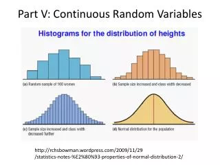
5.4: Descriptive Methods for Assessing Normality • If the data are normal • A histogram or stem-and-leaf display will look like the normal curve • The mean ± s, 2s and 3s will approximate the empirical rule percentages • The ratio of the interquartile range to the standard deviation will be about 1.3 • A normal probability plot , a scatterplot with the ranked data on one axis and the expected z-scores from a standard normal distribution on the other axis, will produce close to a straight line McClave: Statistics, 11th ed. Chapter 5: Continuous Random Variables
5.4: Descriptive Methods for Assessing Normality Errors per MLB team in 2003 • Mean: 106 • Standard Deviation: 17 • IQR: 22 22 out of 30: 73% 28 out of 30: 93% 30 out of 30: 100% McClave: Statistics, 11th ed. Chapter 5: Continuous Random Variables
5.4: Descriptive Methods for Assessing Normality A normal probability plot is a scatterplot with the ranked data on one axis and the expected z-scores from a standard normal distribution on the other axis McClave: Statistics, 11th ed. Chapter 5: Continuous Random Variables
EXAMPLE 5.11 CHECKING FOR NORMAL DATA—EPA Estimated Gas Mileages Problem The EPA mileage ratings on 100 cars, first presented in Chapter 2 (p. 38), are reproduced in Table 5.2. Numerical and graphical descriptive measures for the data are shown on the MINITAB and SPSS printouts presented in Figure 5.18a–c. Determine whether the EPA mileage ratings are from an approximate normal distribution.