Download
1 / 48
480 likes | 622 Views
11-F Scaling Function. 定義 scaling function 為. where. for f > 0, ( − f ) = *( f ). ( t ) is usually a lowpass filter (Why?). 修正型的 Wavelet transform. (1). a is any real number , 0 < b < b 0. (2). reconstruction:. 由 b 0 至 ∞ 的積分被第二項取代. (Proof): If.

E N D
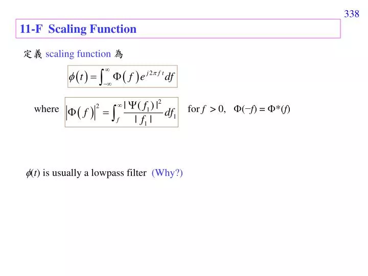
11-F Scaling Function 定義 scaling function為 where for f > 0, (−f) = *(f) (t) is usually a lowpass filter (Why?)
修正型的 Wavelet transform (1) a is any real number, 0 < b < b0 (2) reconstruction: 由 b0至 ∞ 的積分被第二項取代
(Proof): If (from the similar process on pages 334 and 335) 關鍵
Therefore, if y(t) = y1(t) + y2(t), y(t) = x(t)
11-GProperty (1) real input real output (2) If x(t) Xw(a, b), then x(t− ) Xw(a −, b), (3) If x(t) Xw(a, b), then x(t /) (4) Parseval’s Theory: When (t) = C−1(t),
11-H Scalogram Scalogram 即 Wavelet transform 的絕對值平方 有時,會將 Scalogram 定義成
11-I Problems Problems of the continuous WT (1) hard to implement (2) hard to find (t) Continuous WT is good in mathematics. In practical, the discrete WT and the continuous WT with discrete coefficients are more useful.
XII. Continuous WT with Discrete Coefficients 12-A 定義 The parameters a and b are not chosen arbitrarily. For example, a = n2m and b = 2m. 註:某些文獻把這個式子稱作是 discrete wavelet transform,實際上仍然是continuous wavelet transform 的特例 Main reason for constrain a and b to be n2m and 2m : Easy to implementation Xw(n, m) can be computed from Xw(n, m−1) bydigital convolution.
12-BInverse Wavelet Transform 1(t) is the dual function of (t). i.e., should be satisfied.
We often desire that 1(t) = (t). The mother wavelet should satisfies
12-C Haar Wavelet (t) mother wavelet (wavelet function) (t) scaling function 1 t=0 t= 0.5 t=1 t = 1 t = 0 (2t) (2t) 2(2t) = (t) + (t) 0 0.5 (t) = (2t) + (2t–1) (t) = (2t) – (2t–1)
(2mt − n) (2mt − n) t=n2-m t=(n+.5)2-m t=(n+1)2-m t=n2-m t=(n+1)2-m Advantages of Haar wavelet (1) Simple (2) Fast algorithm (3) Orthogonal →reversible (4) Compact, real, odd (5) Vanish moment
Properties (1) 任何 function 都可以由 (t), (2t), (4t), (8t), (16t), ……….. 以及它們的位移所組成 (2) 任何平均為 0的function 都可以由 (t), (2t), (4t), (8t), (16t), ……….. 所組成 換句話說……. 任何 function 都可以由 constant, (t), (2t), (4t), (8t), (16t), ……….. 所組成
(3) Orthogonal The dual function of (t) is (t) itself.
(4) 不同寬度 (也就是不同 m) 的 wavelet / scaling functions 之間會有一個關係 (t) = (2t) + (2t − 1) (t − n) = (2t − 2n) + (2t − 2n − 1) (2mt − n) = (2m+1t − 2n) + (2m+1t − 2n − 1) (t) = (2t) − (2t − 1) (t − n) = (2t − 2n) − (2t − 2n − 1) (2mt − n) = (2m+1t − 2n) − (2m+1t − 2n − 1)
layer: w[n, m] w[2n, m +1] w[4n, m +2] w[4n+1, m +2] Xw[2n, m +1] −1 w[2n+1, m+1] Xw[n, m] w[4n+2, m +2] −1 Xw[2n+1, m +1] w[4n+3, m +2] −1 structure of multiresolution analysis (MRA)
12-D General Methods to Define the Mother Wavelet and the Scaling Function Constraints: (a) near compact support (b) fast algorithm (c) real (d) vanish moment (e) orthogonal 和 continuous wavelet transform 比較: (1) compact support 放寬為 “near compact support” (2) 沒有 even, odd symmetric 的限制 (3) 由於只要是 orthogonal, 必定可以 reconstruction 所以不需要 admissibility criterion 的限制 (4) 多了對 fast algorithm 的要求
12-E Fast Algorithm Constraints Higher and low resolutions 的 recursive relation 的一般化 稱作 dilation equation (t): mother wavelet, (t): scaling function 這些關係式成立,才有fast algorithms
If then If then
(Step 1) convolution (Step 2) down sampling
2 2 m越大,越屬於細節
To satisfy , FT FT where (f) 是 (t) 的 continuous Fourier transform G(f) 是 {gk} 的 discrete time Fourier transform
連乘 (可以藉由 normalization, 讓 (0) = 1) 若G(f) 決定了,則 (f) 可以被算出來 G(f): 被稱作generating function constraint 1
同理 constraint 2 另外,由於 (f = 0 代入) 必需滿足 constraint 3
12-F Real Coefficient Constraints Since If are satisfied, constraint 4 constraint 5 then (f) = *(− f),(f) = *(−f), and (t), (t) are real. Note: If these constraints are satisfied,gk, hkon page 356 are also real.
12-G Vanish Moment Constraint If (t) has p vanishing moments, for k = 0, 1, 2, …, p−1 Since from the Parseval’s Theorem, (Here, we use the fact that general form of the sifting property )
Therefore, Taking the conjugation on both sides, Since if for k = 0, 1, 2, …, p−1 is satisfied, constraint 6 then for k = 0, 1, 2, …, p−1 are satisfied and the wavelet function has p vanishing moments.
12-H Orthogonality Constraints orthogonality constraint: (t): wavelet function If the above equality is satisfied, forward wavelet transform: inverse wavelet transform: (much easier for inverse) C = mean of x(t) (證明於後頁)
If and then due to
Therefore, is the inverse operation of #
※ 要滿足 之前,需要滿足以下三個條件 (1) 這個條件若滿足, 對所有的 m皆成立 (2) for scaling function 嚴格來說,這並不是必要條件,但是可以簡化 第 (3) 個條件的計算
(3) for any n, n1 if k > 0 若 (1) 和 (3) 的條件滿足,則 也將滿足 (Proof): Set If (3) is satisfied, when m m1 In the case where m= m1, if (1) is satisfied, then #
由 Page 369 的條件 (1) Parseval’s theorem if p is an integer Therefore, for all f should be satisfied
同理,由 Page 369的條件 (2) for scaling function 推導過程類似 page 371 for all f should be satisfied
衍生的條件:將 代入 (page 371) 因為 hk是 discrete sequence, H(f) 是hk的 discrete-time Fourier transform
因為 for all f (page 371的條件) constraint 7
同理,將 代入 (page 371) 經過運算可得 constraint 8
Page 370條件 (3) 的處理 由於 是 的 linear combination 是 的 linear combination 是 的 linear combination : : 是 的 linear combination 所以 必定可以表示成 的 linear combination
所以,若 for any n1, nk可以滿足 則 for any n1, nk必定能夠成立 Page 370 條件 (3) 可改寫成 (將 t−n1變成 t, = nk−n1) (from Parseval’s theorem)
Since (since from page 377, is an integer)
Since Since for all f (page 371) constraint 9
12-I Nine Constraints 整理: 設計 mother wavelet 和 scaling function 的九大條件 (皆由 page 355 的 constraints 衍生而來) (1) for fast algorithm , page 361 (2) for fast algorithm , page 362 (3) for fast algorithm , page 362 for real , page 363 (4) (5) for real , page 363 (6) for p vanish moments , page 365 for k = 0, 1, …, p-1
(7) for orthogonal , page 364 for orthogonal , page 365 (8) for orthogonal , page 369 (9)
條件的簡化 有時,令 此時,若 (條件 (5), (8) 滿足) 則 條件 (4), (7), (9) 也將滿足
整理: 設計 mother wavelet 和 scaling function 的幾個要求 (簡化版) (1) for fast algorithm (2) for fast algorithm (3) for fast algorithm (4) for real for p vanish moments (5) for k = 0, 1, …, p-1 (6) for orthogonal (7)
附錄十二 幾種常見的影像壓縮格式 (1) JPEG: 使用 discrete cosine transform (DCT) 和 88 blocks是當前最常用的壓縮格式 (副檔名為 *.jpg 的圖檔都是用 JPEG 來壓縮) 可將圖檔資料量壓縮至原來的 1/8 (對灰階影像而言) 或 1/16 (對彩色影像而言) (2) JPEG2000: 使用 discrete wavelet transform (DWT)壓縮率是 JPEG 的 2~3 倍之間 (3) JPEG-LS: 是一種 lossless compression壓縮率較低,但是可以完全重建原來的影像 (4) JBIG: 針對 bi-level image (非黑即白的影像) 設計的壓縮格式
(5) GIF:使用 LZW (Lempel–Ziv–Welch) algorithm (類似字典的建構) 適合卡通圖案和動畫製作,lossless (6) PNG:使用 LZ77 algorithm (類似字典的建構,並使用 sliding window) lossless (7) JPEG XR (又稱 HD Photo): 使用 Integer DCT,lossless在 lossy compression 的情形下壓縮率可和 JPEG 2000 差不多 (8) TIFF:使用標籤,最初是為圖形的印刷和掃描而設計的,lossless