Download
1 / 20
220 likes | 417 Views
傅思維. Image De-Noising by Wavelet Transform . Introduction to Wavelet transform. How to implement?. g[n]: low pass filter h[n]: high pass filter. :down sampling. Introduction to Wavelet transform. Different sub-bands:.

E N D
傅思維 Image De-Noising by Wavelet Transform
Introduction to Wavelet transform How to implement? g[n]: low pass filter h[n]: high pass filter :down sampling
Introduction to Wavelet transform Different sub-bands: Fig. 2 (a) One level and (b) two level 2-D DWT.
Introduction to Wavelet transform • 1. Localized both in time (space) and frequency domain. • 2. Multiresolution analysis (MRA). Ex:
Why wavelet? • Traditional Fourier transform:
Flowchart of wavelet de-noising: 1. Perform the DWT on the noisy image to obtain sub-bands. 2. Threshold all high frequency sub band coefficients using certain thresholdingmethod. 3. Perform the inverse DWT to reconstruct the de-noised Image.
Two thresholding methods: Hard-thresholding: • f_h(x) = x if abs(x) ≥ λ (1) = 0 otherwise Soft-thresholding: • f_s(x) = x −λ if x ≥ λ = 0 if x < λ (2) = x +λ if x ≤ −λ
Two thresholding methods: (a) (b) Fig. 3 (a) Hard-thresholding and (b) soft-thresholding
Threshold determination • 1. VisuShrink: T=σ (universal) Where σ is the noise standard deviation and M is the number of pixels in the image. • 2. BayesShrink: TB = (adaptive) Where is the standard deviation of signal. . . .
??? • The noise variance can be estimated from the sub-band HH1 by the robust median estimator: => σ = (Median(|Yij |))/0.6745 Yij ϵ subband HH1 (3) (cited 6800 times!) D. L. Donoho and I. M. Johnstone, “Ideal spatial adaptation via wavelet shrinkage,” Biometrika, vol. 81, pp. 425–455, 1994.
Ex: • 0 -> 2.3743 • 10 -> 10.5174 • 20 -> 20.1602 • 30 -> 30.2146
Additive white Gaussian noise Table I: PSNR of test image corrupted by AWGN Cheat! 1.The standard deviation of the Gaussian lowpass filter is chosen until the best result appears. 2.The window size of Wiener filter is chosen until the best result appears (shown in the parentheses).
Appendix The noise model can be assumed to Y = X + N, with X and N are independent of each other, hence (4) As Y is modeled as zero mean Gaussian, is computed by: = (5) where n m is the size of the subband under consideration. Finally, we can get by (4) as: (6)