Download
1 / 38
380 likes | 499 Views
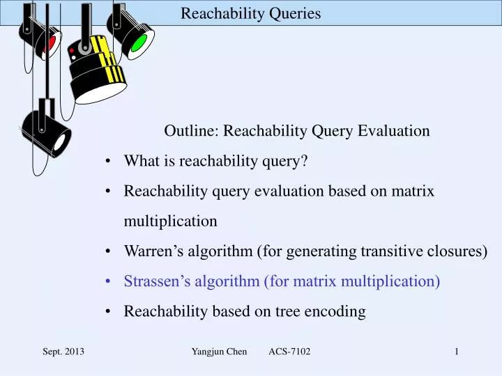
Outline: Reachability Query Evaluation What is reachability query? Reachability query evaluation based on matrix multiplication Warren’s algorithm (for generating transitive closures) Strassen’s algorithm (for matrix multiplication) Reachability based on tree encoding. Motivation.

E N D
Outline: Reachability Query Evaluation • What is reachability query? • Reachability query evaluation based on matrix multiplication • Warren’s algorithm (for generating transitive closures) • Strassen’s algorithm (for matrix multiplication) • Reachability based on tree encoding Yangjun Chen ACS-7102
Motivation • Efficient method to evaluate graph reachability queries • Given a directed graphG, check whether a node v is reachable from another node u through a path in G. • Application • - XML data processing • - Type checking in object-oriented languages and databases • - Geographical navigation • - Internet routing • - CAD/CAM, CASE, office systems, software management Yangjun Chen ACS-7102
a b c d e 1 0 0 0 0 a b c d e 0 0 0 0 0 1 0 0 0 0 1 0 1 0 0 0 0 1 0 0 a a M = c c b b e e d d Motivation • A simple method • - store a transitive closure as a matrix G: G*: The transitive closure G* of a graph G is a graph such that there is an edge (u, v) in G* iff there is path from u to v in G. Yangjun Chen ACS-7102
a c b e d n å a b c d e j=1 0 0 0 0 0 a b c d e 0 0 0 0 0 0 0 0 0 0 1 0 0 0 0 1 0 0 0 0 Matrix Multiplication • Definition • - Two matrices A and B are compatible if the number of columns of A equals the number of B. • - If A = (aij) is an m n matrix and B = (bij) is an n p matrix, then their matrix product C = A B is an m p matrix C = (cik) such that • cik = aijbjk for i = 1, 2, …, m and k = 1, 2, …, p. Each entry (i, j) in M M represents a path of length 2 from i to j. M M = G: Yangjun Chen ACS-7102
Each entry (i, j) in M M represents a path of length 2 from i to j. Each entry (i, j) in M M M represents a path of length 3 from i to j. Each entry (i, j) in M M M … M represents a path of length k from i to j. . . . k Define: M* = M(1) M(2) M(3)… M(n) Each entry (i, j) in M* represents a path from i to j. Time overhead: O(n4). Space overhead: O(n2). Query time: O(1). Yangjun Chen ACS-7102
a b c d e a b c d e 1 0 0 0 0 1 0 0 0 0 a b c d e a b c d e 0 0 0 0 0 0 0 0 0 0 1 0 0 0 0 1 0 0 0 0 1 0 1 0 0 1 0 1 0 0 1 0 1 0 0 0 0 1 0 0 a a c c b b e e d d Example G: M = G*: M* = M (M M) = Each entry (i, j) in P represents a path from i to j. Yangjun Chen ACS-7102
Warren’s Algorithm Warren’s algorithm is a quite simple way to generate a boolean matrix to represent the transitive closure of a graph G. Assume that G is represented by a boolean matrix M in which M(i, j) = 1 if edge (i, j) is in G, and M(i, j) = 0 if (i, j) is not in G. Then, the matrix M’ for the transitive closure of G can be computed from M, in which M’(i, j) = 1 if there exits a path from i to j in G, and M’(i, j) = 0 if there is no path from i to j in G. Warren’s algorithm is given below: AlgorithmWarren fori = 2 to n do forj = 1 to i - 1 do {ifM(i, j) = 1 then set M(i, *) = M(i, *) M(j, *);} fori = 1 to n - 1do forj = i + 1 to ndo {ifM(i, j) = 1 then set M(i, *) = M(i, *) M(j, *);} In the algorithm, M(i, *) denotes row i of M. The theoretic time complexity of Warren’s algorithm is O(n3). Yangjun Chen ACS-7102
i i i j j j k k k x x x ifM(i, j) = 1 then set M(i, *) = M(i, *) M(j, *) i j k x ifM(i, k) = 1 then set M(i, *) = M(i, *) M(k, *) S. Warshall, “A Theorem on Boolean Matrices,” JACM, 9. 1(Jan. 1962), 11 - 12. H.S. Warren, “A Modification of Warshall’s Algorithm for the Transitive Closure of Binary Relations,” Commun. ACM 18, 4 (April 1975), 218 - 220. Yangjun Chen ACS-7102
r t a c e g s u b d f h Strassen’s Algorithm Strassen’s algorithm runs in O(nlg7) = O(n2.81) time. For sufficiently large values of n, it outperforms Warren’s algorithm. • An overview of the algorithm Strassen’s algorithm can be viewed as an application of a familiar design technique: divide and conquer. Consider the computation C = A B, where A, B, and C are n n matrices. Assuming that n is an exact power of 2, we divide each of A, B, and C into four n/2 n/2 matrices, rewriting the equation C = A B as follows: r = ae + bg s = af + bh t = ce + dg u = af + dh = Yangjun Chen ACS-7102
Each of these four equations specifies two multiplications of n/2 n/2 matrices and the addition of their n/2 n/2 products. So the time complexity of the algorithm satisfies the following recursive equation: T(n) = 8T(n/2) + O(n2) The solution of this equation is T(n) = O(n2). Strassen discovered a different approach that requires only 7 recursive multiplications of n/2 n/2 matrices and O(n2) scalar additions and subtractions, yielding the recurrence: T(n) = 7T(n/2) + O(n2) = O(nlg7) = O(n2.81). Yangjun Chen ACS-7102
Strassen’s algorithm works in four steps: • Divide the input matrices A and B into n/2 n/2 matrices. • Using O(n2) scalar additions and subtractions, computer 14 • matrices A1, B1, A2, B2, …, A7, B7, each of which is n/2 n/2. • 3. Recursively compute the seven matrix products Pi = Ai Bi for • i = 1, 2, …, 7. • Computer the desire submatrices r, s, t, u of the result matrix C • by adding and/or subtracting various combinations of the Pi • matrices, using only O(n2) scalar additions and subtraction. A1 = a, A2 = (a + b), A3 = (c + d), A4 = d, A5 = (a + d), A6 = (b – d), A7 = (c – a) B1 = (f –h), B2 = h, B3 = e, B4 = (g – d), B5 = (e + h), B6 = (g + h), B7 = (e + f) r= ae + bg = P5 + P4 - P2 + P6,s= af + bh = P1 + P2, t= ce + dg = P3 + P4,u= af + dh = P5 + P1 – P3 + P7. 7 matrix multiplication, 18 matrix additions and subtractions. Yangjun Chen ACS-7102
Assume that n = 2m. We have T(2m) = 7T(2m-1) + 18(2m-1)2. Am = 7Am-1 + 18(2m-1)2, A1 = 18. G(x) = A1 + A2x + A3x2 + … = A1 + (7A1 + 1822)x + (7A2 + 1823)x2 … … = 18 + 7x G(x) + 184x/(1 – 4x) (1 - 7x)G(x) = 18(4x/(1 – 4x) + 1) = 18/(1 – 4x) Yangjun Chen ACS-7102
G(x) = 18/(1 – 4x)(1 – 7x) = 18 G(x) = 6 (7k+1 – 4k+1)xk 7/3 -4/3 ( ) + 1 – 7x 1 – 4x log2n log27 = O(67 ) = O(6n ) å k=0 (1 - 7x)G(x) = 18(4x/(1 – 4x) + 1) = 18/(1 – 4x) Am = 6(7m – 4m), m = log2n = O(n2.81) Yangjun Chen ACS-7102
Determining the submatrix products It is not clear exactly how Strassen discovered the submatrix products that are the key to making his algorithm work. Here, we reconstruct one plausible discovery method. Write Pi = Ai Bi = (i1a + i2b + i3c + i4d) (i2e + i1f + i3g + i4h), where the coefficients ij, ijare all drawn from the set {-1, 0, 1}. We guess that each product is computed by adding or subtracting some of the submatrices of A, adding or subtracting some of submatrices of B, and then multiplying the two results together. Yangjun Chen ACS-7102
Pi = Ai Bi = (i1a + i2b + i3c + i4d) (i1e + i2f + i3g + i4h) i1 i2 i3 i4 e f g h = (a b c d) (i1 i2 i3 i4) i1i1 i1i2 i1i3 i1i4 i2i1 i2i2 i2i3 i2i4 i3i1 i3i2 i3i3 i3i4 i4 i1 i4i2 i4i3 i4i4 e f g h = (a b c d) Yangjun Chen ACS-7102
+1 0 0 0 0 0 +1 0 0 0 0 0 0 0 0 0 r t a c e g s u b d f h r = ae + bg s = af + bh t = ce + dg u = af + dh = r = ae + bg So r is represented by a matrix: + + e f g h = (a b c d) ‘’ – represents 0. ‘+’ – represents +1. ‘-’ – represents -1. Yangjun Chen ACS-7102
s = af + bh t = ce + dg s = cf + dh + + + + + + = = = We will create 7 matrices in such a way that the above 4 matrices can be generated by addition and subtraction operations over these 7 matrices. Furthermore, the 7 matrices themselves can be produced by 7 multiplications and some additions and subtractions. Yangjun Chen ACS-7102
P1= A1B1 = a·(f – h) = af - ah P2= A2B2 = (a + b) h = ah + bh s = af + bh +- + + + + = = = = P1 + P2 Yangjun Chen ACS-7102
P3= A3B3 = (c + d) e = ce + de P4= A4B4 = d (g - e) = dg - de t = ce + dg + + + + -+ = = = = P3 + P4 Yangjun Chen ACS-7102
P5= A5B5 = (a + d) (e + h) = ae + ah + de + dh P6= A6B6 = (b – d)(g + h) = bg + bh – dg - dh + + ++ ++ -- = = r = ae + bg + + = P5 + P4 – P2 + P6 = Yangjun Chen ACS-7102
P7= A7B7 = (a - c) (e + f) = ae + af - ce - cf + + -- = u = cf + dh + + = P5 + P1 – P3 – P7 = Yangjun Chen ACS-7102
Tree encoding • Definition • - We can assign each node v in a tree T an interval [v, v), where vis v’s preorder number (denoted pre(v)) and v- 1 is equal to the largest preorder number among all the nodes in T[v] (subtree rooted at v). • - So another node u labeled [u, u) is a descendant of v (with respect to T)iff u [v, v). • - If u [v, v), we say, [u, u) is subsumed by [v, v). This method is called the tree labeling. Yangjun Chen ACS-7102
Example: a [0, 13) h b [10, 13) r [6, 10) [1, 6) d c j i [2, 5) [7, 10) e [5, 6) [11, 12) [12, 13) p [3, 5) [8, 9) [9, 10) g f k [4, 5) Yangjun Chen ACS-7102
Reachability checking based on tree encoding Directed acyclic graphs (DAGs) - Find a spanning tree T of G, and assign each node v an interval. - Examine all the nodes in G in reverse topological order and do the following: For every edge (p, q), add all the intervals associated with the node q to the intervals associated with the node p. When adding an interval [i, j) to the interval sequence associated with a node, if an interval [i’, j’) is subsumed by [i, j), it will be discarded from the sequence. In other words: if i’ [i, j), then discard [i’, j’]. On the other hand, if an interval [i’, j’) is equal to [i, j) or subsumes [i, j). [i, j) will not be added to the sequence. Otherwise, [i, j) will be inserted. Yangjun Chen ACS-7102
Topological order of a directed acyclic graph: Linear ordering of the vertices of G such that if (u, v) E, then u appears somewhere before v. Example: a [0, 13) h b [10, 13) r [6, 10) [1, 6) c j d i [2, 5) [7, 10) e [5, 6) [11, 12) [12, 13) p g [3, 5) [8, 9) f [9, 10) k [4, 5) Topological order: a, b, r, h, e, f, g, d, c, p, k, i, j Yangjun Chen ACS-7102
Reverse topological order: A sequence of the nodes of G such that for anyedge (u, v) v appears before u in the sequence. k, p, c, d, f, g, i, j, e, r, b, h, a Reverse topological order a [0, 13) L(k) = [4, 5) L(p) = [3, 5) L(c) = [2, 5) L(d) = [4, 5)[5, 6) L(f) = [4, 5)[5, 6)[8, 9) L(g) = [2, 5)[5, 6)[9, 10) L(i) = [11, 12) L(j) = [12, 13) L(e) = [2, 5)[5, 6)[7, 10) L(r) = [2, 5)[5, 6)[6, 10) L(b) = [1, 6) L(h) = [4, 5)[7, 10)[10, 13) L(a) = [10, 13) h b [10, 13) r [6, 10) [1, 6) c j d i [2, 5) [7, 10) e [5, 6) [11, 12) [12, 13) p [3, 5) g [8, 9) f k [4, 5) [9, 10) Yangjun Chen ACS-7102
Generation of interval sequences • First of all, we notice that each leaf node is exactly associated with • one interval, which is trivially sorted. • Let v1, ..., vl be the child nodes of v, associated with the interval • sequences L1, ..., Ll, respectively. • Assume that the intervals in each Li are sorted according to the first element in each interval. We will merge all Li’s into the interval sequence associated L with v as follows. • Let [a1, b1) (from L) and [a2, b2) (from Li) be the interval • encountered. We will perform the following checkings: Yangjun Chen ACS-7102
L = [a1, b1) … Li= [a2, b2) … • Ifa2 >= a1then • {if a2 [a1, b1) then go to the interval next to [a2, b2) and compare it • with [a1, b1) in a next step • else go to the interval next to [a1, b1) and compare it • with [a2, b2) in a next step.} • If a1 > a2then • {if a1 [a2, b2) then remove [a1, b1) from L and compare the interval • next to [a1, b1) with [a2, b2) in a next step • else insert [a2, b2) into L before [a1, b1).} • Obviously, |L| b (the number of the leaf nodes in the spanning tree T)and the • intervals in L are sorted. The time spent on this process is O(dvb), where dv • represents the outdegree of v. So the whole cost • is bounded by • O( ) = O(be). Yangjun Chen ACS-7102
Reachability checking for DAGs • Let u and v be two nodes of G. • u is a descendant of v iff there exists an interval [, )in L(v) such that u [, ). Example: [k, k) = [4, 5) L(r) = [2, 5)[5, 6)[6, 10) Node k is a descendant of node r. Yangjun Chen ACS-7102
Reachability checking for cyclic graphs • Using Tarjan’s algorithm to recognize all the strongly connected components (SCCs). In each SCC, any two nodes are reachable from each other. • Collapse each SCC to a single node. In this way, any cyclic graph G is transformed to a DAG G’. • Let u and v be to two nodes in G. Check their reachability according to two cases: • u and v are in two different SCC. • u and v are in the same SCC. Yangjun Chen ACS-7102
Using tree encoding as a filter • A different tree encoding • Each node v ina tree T is labeled with a with a range • Iv = [rx, rv], • where rv is the postorder number of v (the postorder numbers are assumed to begin at 1) and rx is the lowest postorder number of any node x in the subtree rooted at v (i.e., including v). • This approach guarantees that the containment between intervals is equivalent to the reachability relationship between the nodes, since the postorder traversal enters a node before all of its descendants have been visited. • In other words, u ↝ v Iv Iu. Yangjun Chen ACS-7102
[1,10] 0 [1,6] [7,9] 1 2 [5,5] [1,4] [7,8] 3 4 5 [7,7] [1,3] 6 7 [2,2] [1,1] 8 9 Example: The above figure shows the interval labeling on a tree, assuming that the children are ordered from left to right. It is easy to see that reachability can be answered by interval containment. For example, 1 ↝ 9, since I9 = [2, 2] ⊂ [1, 6] = I1, but 2 ↝ 7, since I7 = [1, 3] [7, 9] = I2. Yangjun Chen ACS-7102
[1,10] 0 [1,6] [7,9] 1 2 [5,5] [1,4] [7,8] 3 4 5 [7,7] [1,3] 6 7 [1,10] [2,2] 0 [1,1] 8 9 [1,6] [1,9] 1 2 [1,5] [1,4] [1,8] 3 4 5 [1,7] [1,3] 6 7 [2,2] [1,1] 8 9 Using tree encoding as a filter To generalize the interval labeling to a DAG G, we have to ensure that a node is not visited more than once, and a node will keep the postorder number of its first visit. That is, in [rx, rv], rv is produced by exploring G bottom-up. However, rx is now the lowest postorder number of any node x the sub-graph rooted at v. Yangjun Chen ACS-7102
The above shows an interval labeling on a DAG, assuming a left to right ordering of the children. As one can see, interval containment of nodes in a DAG is not exactly equivalent to reachability. For example, 5 ↝ 4, but I4 = [1, 5] ⊆ [1, 8] = I5. In other words, Iv ⊆ Iu does not imply that u ↝ v. On the other hand, one can show that Iv Iu ⇒ u ↝v. [1,10] 0 [1,6] [1,9] 1 2 [1,5] [1,4] [1,8] 3 4 5 [1,7] [1,3] 6 7 [2,2] [1,1] 8 9 Yangjun Chen ACS-7102
[1,10], [1, 10] 0 [1,6], [1, 9] [1,9], [1, 7] 1 2 [1,5], [1, 8] [1,4], [1, 6] [1,8], [1, 3] 3 4 5 [1,7], [1, 2] [1,3], [1, 5] 6 7 [2,2], [4, 4] [1,1], [1, 1] 8 9 • Instead of using a single interval, one can employs multiple intervals • that are obtained via random graph traversals. • We use the symbol d to denote the number of intervals to keep per • node, which also corresponds to the number of graph traversals used • to obtain the label. • The following figure shows a DAG labeling using 2 intervals • (the first interval assumes a left-to-right ordering of the children, • whereas the second interval assumes a right-to-left ordering). [1, 10] 0 [1, 9] [1, 7] 1 2 [1, 6] [1, 3] [1, 8] 3 4 5 [1, 2] [1, 5] 6 7 8 9 [4, 4] [1, 1] Yangjun Chen ACS-7102
Index construction An interval Iui is denoted as Iui = [Iui[1], Iui[2] ] = [rx, ru] Algorithm 1: Randomized Intervals RandomizedLabeling(G, d): 1 foreachi ← 1 to ddo //d – number of intervals for each node 2 r ← 1 // global variable: postorder number of node 3 Roots ← {n : n∈ roots(G)} 4 foreachx ∈ Roots in random orderdo 5 Call RandomizedVisit(x, i, G) RandomizedVisit(x, i, G) : 6 ifxvisited beforethen return 7 foreachy ∈ Children(x) in random orderdo 8 Call RandomizedVisit(y, i, G) 9 rc*← min{Ici[1] : c ∈ Children(x)} 10 Ixi ← [min(r, rc*), r] 11 r ← r + 1 Yangjun Chen ACS-7102
Reachability queries • To answer reachability queries between two nodes, u and v, • we will first check whether IvIu. If so, we can immediately • conclude that u ↝ v. • On the other hand, if Iv ⊆ Iu, nothing can be concluded • immediately since we know that the index can have false positives, • i.e., exceptions. In this case, a DFS (depth-first search) is • conducted, with recursive containment check based pruning, • to answer queries. In the worst case, it needs O(n) time. Another • way is to check the exception lists associated with the nodes: Ex = {y : (x, y) is an exception, i.e., Iy⊆ Ix and x ↝y}. Yangjun Chen ACS-7102
DFS with prunning Algorithm 2: Reachability Testing Reachable(u, v, G): 1 ifIvIuthen 2 returnFalse // u↝v 3 else if use exception lists then 4 ifv ∈ EuthenreturnFalse // u↝ v 5 elsereturnTrue // u↝ v 6 else // DFS with pruning 7 foreach cChildren(u) such thatIv ⊆ Icdo 8 ifReachable(c, v, G) then 9 returnTrue // u ↝ v 10 returnFalse // u ↝ v Yangjun Chen ACS-7102