Download

1 / 126
1.31k likes | 1.49k Views
MEDICAL DECISION MAKING. Dr. Ali M. Hadianfard (Medical Informatics) Faculty member of AJUMS (paramedical school) http:// www.alihadianfard.info / download.html. Further reading.

E N D
MEDICAL DECISION MAKING Dr. Ali M. Hadianfard (Medical Informatics) Faculty member of AJUMS (paramedical school) http://www.alihadianfard.info/download.html
Further reading Biomedical Informatics-Computer Applications in Health Care and Biomedicine, Edward H. Shortliffe, James J. Cimino, 4th Ed., 2014 (chapter 3 & 22). Decision Support Systems and Intelligent Systems, EfraimLiang,Ting-Peng Aronson, Jay E. Turban, 7th Ed., 2004 (chapter 2). Medical Decision Making, Harold C. Sox, Michael C.Higgins, Douglas K. Owens, 2nd Ed., 2013 (chapters 3, 5 & 6). From Patient Data to Medical Knowledge The Principles and Practice of Health Informatics, Paul_Taylor, 2006 (chapter 10). Clinical Decision Support Systems Theory and Practice Health Informatics, Eta S. Berner, 2nd Ed., 2006 (chapters 1 & 2). Fuzzy control and identification, John. Lilly, 2010 (chapters 1 & 2).
What is Medical Informatics? The study of applying computer technology to manage medical information in order to affect medical care and support problem-solving and decision-making.
Decision-making Can be considered as the cognitive process (the thought process) selecting a logical choice from the available alternatives. Common examples include shopping, deciding what to eat, and deciding whom or what to vote for in anelection or referendum.
Problem-solving A problem occurs when a system does not meet its established goals, does not yield the predicted results, or does not work as planned. Problem-solving may also deal with identifying new opportunities. Sometimes the terms decision-making and problem-solving are used interchangeably.
Decision-making process (1) Simon's model (1977) is the most concise and yet complete characterization of rational decision-making. This involves three major phases: Intelligence, Design, and Choice. He later added a fourth phase, Implementation. Monitoringcan be considered a fifth phase.
Decision-making process (2) Intelligence phase: Scanning the environment Data collection (objectives) Problem identification Problem ownership ( at the national or international levels or a problem exists in an organization only if someone or some group takes on the responsibility of attacking it and if the organization has the ability to solve it) Problem classification (definable category, well-structured problems, unstructured problems ) Problem statement
Decision-making process (3) Design phase: These include understanding the problem and testing solutions for feasibility. A model of the decision-making problem is constructed, tested, and validated Formulate a model based on the relationships among all the variables (Modeling involves conceptualizing the problem and abstracting it to quantitative and/or qualitative form. For a mathematical model, the variables are identified and their mutual relationships are established) Validate of the model Set criteria for choice Search for alternatives Predict and measure outcomes
Decision-making process (4) Choice phase: Selection of a proposed solution to the model, Selection of best (good) alternative(s) Plan for implementation The solution is tested to determine its viability and profitability The boundary between the design and choice phases is often unclear because certain activities can be performed during both of them and because one can return frequently from choice activities to design activities. For example, one can generate new alternatives while performing an evaluation of existing ones.
Decision-making process (5) Implementation phase: Once the proposed solution seems reasonable, we are ready for the last phase: implementation of the decision. implementation means putting a recommended solution to work. Successful implementation results in solving the real problem. Failure leads to a return to an earlier phase of the process. In fact, we can return to an earlier phase during any of the latter three phases.
Decision-making under different conditions • Certainty: • There is perfect knowledge of all the information needed to make a decision. • Problems are structured • Solutions are already available from past experiences • Risk: • Information is incomplete • The problem and the alternatives are defined, but has no guarantee how each solution will work. • It is feasible to make a list of all possible outcomes and assign probabilities to the various outcomes. • Uncertainty: • information is very poor • Problems are unstructured • Decision maker cannot list all possible outcomes and/or cannot assign probabilities to the various outcomes.
Medical Decision Making is under Uncertainty Decision making is one of the quintessential activities of the healthcare professional. Some decisions are made on the basis of deductive (subtract from a total; antonym: inductive ) reasoning or of physiological principles. Many decisions, however, are made on the basis of knowledge that has been gained through collective experience: the clinician often must rely on empirical knowledge of associations between symptoms and disease to evaluate a problem. A decision that is based on these usually imperfect associations will be, to some degree, uncertain. Clinical data are imperfect. The degree of imperfection varies, but all clinical data—including the results of diagnostic tests, the history given by the patient, and the findings on physical examination— are uncertain.
Example: uncertain condition Mr. James is a 59-year-old man with coronary artery disease. The patient often experiences chest pain (angina). Mr. James has twice undergone coronary artery bypass graft (CABG) surgery. Unfortunately, he has again begun to have chest pain, which becomes progressively more severe, despite medication. If the heart muscle is deprived of oxygen, the result can be a heart attack (myocardial infarction), in which a section of the muscle dies. Should Mr. James undergo a third operation? The medications are not working; without surgery, he runs a high risk of suffering a heart attack, which may be fatal. On the other hand, the surgery is hazardous. Not only is the surgical mortality rate for a third operation higher than that for a first or second one but also the chance that surgery will relieve the chest pain is lower than that for a first operation. All choices in the example entail considerable uncertainty. Furthermore, the risks are grave; an incorrect decision may substantially increase the chance that Mr. James will die. The decision will be difficult even for experienced clinicians. The use of probability or odds as an expression of uncertainty avoids the ambiguities inherent in common descriptive terms.
Probability Probability is represented numerically by a number between 0 and 1. Statements with a probability of 0 are false. Statements with a probability of 1 are true. An event that is certain to occur has a probability of 1; an event that is certain not to occur has a probability of 0. probability of 0.5 or 50% are just as likely to be true as false. The probability of event A is written p[A]. The sum of the probabilities of all possible, collectively exhaustive outcomes of a chance event must be equal to 1. e.g., p[heads]+ p[tails] = 1.0. Probabilities can be combined to yield new probabilities. and: p[A∩B] = p[A] p[B] or: p[A U B] = p[A] +p[B]
Conditional Probability p[A∩B] = p[A] p[B|A] (Bayes’ theorem) The probability that event A will occur given that event B is known to occur is called the conditional probability of event A given event B, denoted by p[A|B] and read as “the probability of A given B.” Thus a post-test probability is a conditional probability predicated on the test or finding. For example, if 30 % of patients who have a swollen leg have a blood clot, we say the probability of a blood clot given a swollen leg is 0.3, denoted: p[blood clot | swollen leg] = 0.3.
Odds where p is the probability that the event will occur The ratio of the probability of an event occurring over the probability of the event not occurring. Odds and probability are equivalent. The relationship between the odds of an event and its probability is the following: For example, if the probability of the event is 0.67, the odds of the event are 0.67 divided by 0.33, or 2 to 1. Another way to express the odds of an event is p:(1−p). Thus, writing 2:1 is equivalent to saying ‘‘2 to 1 odds.’’ Some find it especially useful to use odds to express their opinion about very infrequent events (1 to 99 odds, rather than a probability of 0.01) or very common events (99 to 1 odds, rather than a probability of 0.99).
Probability Assessment Probability assessment means asking a person to use a numberto express how strongly he/she believes that an event will occur. • When to estimate probability: If the probability of a disease is very low, doing nothing will be the best choice. Treating without further testing is the best choice if the probability of the target condition is relatively high. Testing (getting more information) is best when the probability of disease is intermediate. • How to estimate probability: • Subjective Probability Assessment • Objective Probability Estimates
Probability Assessment- The source of information 1. Personal experience: When estimating probability, a clinician relies on personal experience with similar events. For example, a surgeon uses her experience with similar patients when she estimates the probability that Mr. Jones will survive an open heart operation. 2. Published experience: Published articles report the frequency of death after surgical procedures. These reports provide an average frequency for a large but not necessarily diverse population, raising questions about its applicability to a specific population. 3. Attributes of the patient: The experienced clinician uses published reports and personal experience to make an estimate that applies to the average patient. She/he then adjusts the estimate upward or downward starting from this average figure if the patient has unusual characteristics that might affect his risk (e.g., advanced age or many chronic conditions).
Subjective Probability Assessment (1) It is based on personal experience. An unconscious mental processes that have been described and studied by cognitive psychologists. These processes are termed cognitive heuristics. A cognitive heuristic is a mental process by which we learn, recall, or process information; we can think of heuristics as rules of thumb (guide or principle based on experience or practice). We may make mistakes in estimating probability in deceptive clinical situations.
Subjective Probability Assessment (2) Three heuristics have been identified as important in estimation of probability: Representativeness. Are judged by the degree to which A is representative of, or similar to, B. For instance, what is the probability that this patient who has a swollen leg belongs to the class of patients who have blood clots? To answer, If the patient has all the classic findings (signs and symptoms) associated with a blood clot, the clinician judges that the patient is highly likely to have a blood clot. Difficulties occur with the use of this heuristic when the disease is rare (very low prior probability, or prevalence). when the clinician’s previous experience with the disease is atypical, thus giving an incorrect mental representation; when the patient’s clinical profile is atypical; and when the probability of certain findings depends on whether other findings are present. (More examples can be found in Medical Decision Making, Harold C. Sox, Michael C.Higgins, Douglas K. Owens, 2nd Ed., 2013, P. 38-44.)
Subjective Probability Assessment (3) Availability. Our estimate of the probability of an event is influenced by the ease with which we remember similar events. Events more easily remembered are judged more probable; this rule is the availability heuristic, and it is often misleading. We remember dramatic, atypical, or emotion-laden events more easily and therefore are likely to overestimate their probability. A clinician who had cared for a patient who had a swollen leg and who then died from a blood clot would vividly remember thrombosis as a cause of a swollen leg. The clinician would remember other causes of swollen legs less easily, and he or she would tend to overestimate the probability of a blood clot in patients with a swollen leg. Anchoring and adjustment. A clinician makes an initial probability estimate (the anchor) and then adjusts the estimate based on further information. For instance, the clinician makes an initial estimate of the probability of heart disease as 0.5. If he or she then learns that all the patient’s brothers had died of heart disease, the clinician should raise the estimate because the patient’s strong family history of heart disease increases the probability that he or she has heart disease, a fact the clinician could ascertain from the literature. The usual mistake is to adjust the initial estimate (the anchor) insufficiently in light of the new information.
Objective Probability Estimates (1) Published research results can serve as a guide for more objective estimates of probabilities. We can use the prevalence of disease in the population or in a subgroup of the population, or clinical prediction rules, to estimate the probability of disease. Estimates of disease prevalence in a defined population often are available in the medical literature. The prevalence of a disease in patients who have in common a symptom, physical finding, or diagnostic test result helps a clinician to diagnose the disease. Symptoms, such as difficulty with urination, or signs, such as a palpable prostate nodule, can be used to place patients into a clinical subgroup in which the probability of disease is known. This approach may be limited by difficulty in placing a patient in the correct clinically defined subgroup, especially if the criteria for classifying patients are ill-defined. A trend has been to develop guidelines, known as clinical prediction rules, to help clinicians assign patients to well-defined subgroups in which the probability of disease is known.
Objective Probability Estimates– Example (2) A medical student evaluates a young man with abdominal pain. She is concerned about the possibility of appendicitis. The pain is present throughout the abdomen and is associated with loose bowel movements. The patient does not have localized abdominal tenderness, fever, or an increased blood leukocyte count. The medical student presents the patient to the chief surgical resident who, to the student’s surprise, discharges the patient from the emergency room. The chief surgical resident knows that the prevalence of appendicitis among self-referred adult males with abdominal pain is only 1%. The student should use this information as a starting point as she uses the patient’s clinical findings to estimate the probability of appendicitis. If the history and physical examination do not suggest appendicitis, the probability of appendicitis is very low, since it was 1% in the average patient with abdominal pain. If the examination does suggest appendicitis, the student’s estimate of probability must reflect the low prevalence of appendicitis in all men with abdominal pain.
Objective Probability Estimates (3) Clinical prediction rules are developed from systematic study of patients who have a particular diagnostic problem; they define how clinicians can use combinations of clinical findings to estimate probability. Clinical prediction rules are statistical models of the diagnostic process. The symptoms or signs that make an independent contribution to the probability that a patient has a disease are identified and assigned numerical weights based on statistical analysis(Regression analysis, assigns a numerical weight to each predictor) of the finding’s contribution. The result is a list of symptoms and signs for an individual patient, each with a corresponding numerical contribution to a total score (Discriminant Score). The total score places a patient in a subgroup with a known probability of disease.
Clinical prediction rules – Example Ms. Troy, a 65-year-old woman who had heart attack 4 months ago, has abnormal heart rhythm (arrhythmia), is in poor medical condition, and is about to undergo elective surgery. What is the probability that Ms. Troy will suffer a cardiac complication? Table 3.1 lists clinical findings and their corresponding diagnostic weights. We add the diagnostic weights for each of the patient’s clinical findings to obtain the total score. The total score places the patient in a group with a defined probability of cardiac complications, as shown in Table 3.2. Ms. Troy receives a score of 20; thus, the clinician can estimate that the patient has a 27 % chance of developing a severe cardiac complication.
Recursive partitioning Recursive partitioning is a statistical process that leads to an algorithmfor classifying patients. In recursive partitioning, the diagnostic process is represented by a series of yes–no decision points. If a patient has a finding, he is placed in one group; if not, he is placed in a second group. Each of the two groups resulting from the first yes–no decision point is subjected to a second yes–no question about another finding. The process continues until it reaches a pre-defined stopping point. The goal of the process is to place each patient into a group in which the prevalence of disease is either very high or very low. Typically, the finding that is used at each yes–no decision point is the one that best discriminates between the diseased and non-diseased patients at that point in the partitioning process.
Recursive partitioning – Example A modified version of recursive partitioning was used to categorize adults with a sore throat as having a high, medium, or low probability of having a beta hemolytic streptococcal infection (Figure 3.8). According to some authors, patients with a high likelihood of infection should have treatment without obtaining a throat culture. In patients with a low likelihood of infection, neither throat culture nor treatment may be indicated.
Decision Tree http://www.alihadianfard.info/download.html
Decision Tree The decision tree, a method for representing and comparing the expected outcomes of each decision alternative. It is one way to display an algorithm. It can be used when the outcomes are uncertain, e.g. the results of a surgical operation are unknown. This technique help clinicians to clarify the decision problem and thus to choose the alternative that is most likely to help the patient. Example: There are two available therapies for a fatal illness. The length of a patient’s life after either therapy is unpredictable, as illustrated by the frequency distribution shown in Fig. 3.6 and summarized in Table 3.5. Each therapy is associated with uncertainty: regardless of which therapy a patient receives, he will die by the end of the fourth year, but there is no way to know which year will be the patient’s last. Figure 3.6 shows that survival until the fourth year is more likely with therapy B, but the patient might die in the first year with therapy B or might survive to the fourth year with therapy A. Which of the two therapies is preferable?
Decision tree - component A decision tree diagram consists of 3 types of nodes: Decision nodes - commonly represented by squares Chance nodes - represented by circles End (terminal) nodes or Outcomes - represented by triangles or solid circles A chance node is shown as a circle from which several lines emanate. Each line represents one of the possible outcomes.
The example of decision tree – A chance-node The outcome of a chance event, unknowable for the individual, can be represented by the expected value at the chance node.
Decision Tree – Expected-value Decision Making Calculating Expected Value: The term expected value is used to characterize a chance event, such as the outcome of a therapy. If the outcomes of a therapy are measured in units of duration of survival, units of sense of well-being, or dollars, the therapy is characterized by the expected duration of survival, expected sense of well-being, or expected monetary cost that it will confer on, or incur for, the patient, respectively. To use expected-value decision making, we follow this strategy when there are therapy choices with uncertain outcomes: (1) calculate the expected value of each decision alternative and then (2) pick the alternative with the highest expected value.
Calculating Expected Value – Example 1 We use the average duration of life after therapy (survival) as a criterion for choosing among therapies. The first step we take in calculating the mean survival for a therapy is to divide the population receiving the therapy into groups of patients who have similar survival rates. Then, we multiply the survival time in each group by the fraction of the total population in that group. Finally, we sum these products over all possible survival values. Mean survival for therapy A A = (0.2 × 1) + (0.4 × 2) + (0.3 × 3) + (0.1 × 4) = 2.3 years. Mean survival for therapy B B = (0.05 × 1) + (0.15 × 2) + (0.45 × 3) + (0.35 × 4) = 3.1 years. we should select therapy B.
Calculating Expected Value – Example 2 The person who faced this decision was a 60-year-old man we will call ‘‘Hank.’’ Hank had a history of eczema. Because of this chronic condition, he was unconcerned when a rash first appeared near his anus. However, the persistent discomfort eventually led Hank to seek medical attention. His dermatologist performed a biopsy, which showed that a rare skin cancer, called perianal Paget’s disease, was causing Hank’s newly discovered rash. This disease starts in the epidermis but often will metastasize. Therefore, the dermatologist referred Hank to an oncologist for treatment. First treatment alternative – traditional surgery: In this case the Hank would lose the function of his rectum and be forced to live the remainder of his life with a colostomy bag. Second treatment alternative – microscopically directed surgery: the resections might stop short of the anal mucosa, thereby avoiding the risk of a colostomy. Third treatment alternative – do nothing: This alternative would leave him with untreated local disease, which ultimately could result in an invasive cancer, metastases, and death.
Expected value analysis only captures that single aspect of what can happen to Hank – the length of his life. It ignores the impact of the decision on other factors, such as his quality of life.
Sensitivity Analysis Is the systematic exploration of how the value of one or more parameters will affect the decision-making implications of a model. This tool can support the validity of decision analysis by revealing how changes in the probabilities will affect the conclusions of the analysis.
Folding Back: A decision tree when the problem includes more than one decision node
Algorithm for folding back a decision tree 1. Start with the most distal nodes. 2. Replace each chance node with its expected value p1y1 + p2y2 + p3y3 + . . . + pNyN where p1, p2, p3, . . . , pNare the probabilities for the possible outcomes and y1, y2, y3, . . . , yNare the corresponding values associated with the outcomes. 3.Replace each decision node with the maximum expected value for the possible alternatives Maximum of x1, x2, x3, . . . , xM where x1, x2, x3, . . . , xMare the expected values for the possible alternatives. 4.Repeat until the initial node is reached.