Download
1 / 34
340 likes | 346 Views
SKA System Overview (and some challenges) P. Dewdney Mar 22, 2010. SKA Array & Receptor Technologies. Dense Aperture Arrays. Dishes. 3-Core Central Region. Wide Band Single Pixel Feeds. Sparse Aperture Arrays. Phased Array Feeds. Artists’ Renditions from Swinburne Astronomy Productions.

E N D
SKA System Overview(and some challenges)P. DewdneyMar 22, 2010
SKA Array & Receptor Technologies Dense Aperture Arrays Dishes 3-Core Central Region Wide Band Single Pixel Feeds Sparse Aperture Arrays Phased Array Feeds Artists’ Renditions from Swinburne Astronomy Productions
Sparse aperture arrays for the lowest frequencies LWA (USA) LOFAR (Netherlands et al) Replication by Industry MWA (USA, Australia)
EMBRACE Prototype for Dense Aperture Arrays Industry already involved in production. First Fringes
ATA 42x6m hydroformed dishes ASKAP CART 36x12m panel dishes 10 m composite prototype Dish Design and Prototyping KAT-7 7 x12m composite dishes Prototype 15 m composite dish
ASKAP chequer board array APERTIF (Astron, NL) DRAO Canada Vivaldi arrays Multi-pixels at mid frequencies withdishes + phased-array-feeds Chequer-board phased array (ASKAP, Australia) Chequer-board phased array (ASKAP, Australia) ASKAP, Australia
Offset design M. Fleming
Mold-Based Production rms error: 0.25 mm Industry Involvement in Production Final Mould Alignment
Systems Analysis System Context External interfaces (E)
u-v Coverage (Configuration Task Force) ~800 km 20 km Millenaar, Bolton et al.
Signal Transport & Networks • Investigations of options for long baselines: • Purchase bandwidth; obtain dark fibre; construct bespoke network? • Routing of fibre between receptors. ~300 km Industry Involvement ~5 km McCool, Grigorescu
Example Signal Processing Overview Industry Involvement ~1018 MACs ~1018 MACs ~1018 MACs (WAG) ~5 x10¹⁷ MACs W. Turner Sparse AAs + 250 Dense AA + 2000 15-m dishes with SPFs
Compute Requirements for Dish-based Version of SKA * From correlator with 105 chans out, ~14000 input data streams, dumped every 200 ms. Industry Involvement Software Development • Algorithms for imaging undergoing rapid changes, especially for the new low frequency instruments (e.g. LOFAR). • SKA may require developing new algorithms (and ultimately code), for calibration and imaging, as well as time-domain research. • Optimisation for multi-core (1000’s) will also be a challenge.
Power Consumption • Through out the SKA, power consumption is a major issue: • On-site • Concentrated loads at the centre. • Distributed loads (100’s of km from centre). • Cooling of equipment is difficult in a desert environment. • Off-site • Probably a large computing load (Concentrated). • Reduction of power consumption and optimisation of the power network will be features of design everywhere. • SKA performance may be power limited.
Imaging Dynamic Range (DR) • Don’t want to build a supersensitive (high A/Tsys or SS) telescope: • then find that it hits a limit after a few hours of integration, which is then irreducible because of systematic errors. • Requirements may vary, but DR is not just an issue for one science program. • High DR is a system issue. • need to consider the whole signal chain, signal processing and imaging as a system. • Current System Specification • 1000 hours integration on a field. • ~74 dB at 1.4 GHz.
Potential Limits to (DR) • Cannot model and calibrate systematic effects (errors) that are not fully understood. • Degrees of Freedom • Cannot solve for more parameters than there is information to support. • Information theory provides a fundamental basis for evaluating combinations of measurements, assumptions, and a-priori information. • Theory originally arose from studies of the amount of information that can be transmitted over a “noisy channel”. • Information theory provides guidance on optimum use of information, but does not provide guidance on actually understanding sources of errors. • Errors with direction-dependency, frequency-dependency or time-dependency add greatly to the number of parameters to be solved for.
Potential Limits to (DR) • Time Variability • All analog systems “drift”. • e.g. Gains of amplifiers are functions of temperature. • e.g. Switching levels and sample intervals in A/D converters vary in complex, non-random ways. • Not everything can be digital: antennas, receivers. • Digital systems do not drift. • But they are subject to bit errors at a low level. • Characteristic system drift times cannot be too short. • Calibration Signal-to-noise • Noise on calibrations imparts noise to images. • Calibrations subject to systematic errors too.
Cost vs DR • For a fixed-cost telescope, we have a fundamental design question: Where to put the money? • Do we design extremely robust sub-systems (antennas, receivers, correlators, etc.), whose characteristics are well-known and stable? • Do we design less expensive sub-systems and put funds into back-end computing instead, to calibrate and correct for upstream defects and time-variable errors? • Major aspect of system design and optimization • Probably have to do both things for an extreme sensitivity telescope. • Must also err on the side of investing in difficult to upgrade sub-systems (e.g. antennas, AA’s).
Chick & Egg How do we qualify the SKA analog components at very high sensitivity (i.e. high DR)? Build the SKA so we can get enough sensitivity to qualify the components. • The purpose of the receptor verification programs is to break the loop, and qualify the receptors in the best way possible. • Must invest in difficult to upgrade sub-systems (e.g. antennas, AA’s) – from previous slide.
Inverse Problem • It’s all about beam characteristics, not the type of receptor. • 74 dB DR specification • For an a priori antenna design this is impossible to meet on its own. • e.g. pointing stability would have to be 25 millionth of a beam. • Recovered pointing should meet the spec. • Fortunately there are powerful modelling & calibration techniques to solve for beam characteristics as system parameters, while simultaneously solving for the image. • Depends on • being able to model systematic effects, • having more equations with measured parameters than unknowns, • signal-to-noise of calibration. • But this does not tell us how to set the antenna specifications. • We will have to start with an informed guess. • Building an antenna for 1.4 GHz using the “usual” specs for 12-15 GHz is a good “rule-of-thumb”.
Approximate Verification Work Flow TDP DVA-1 Program
Beam Measurements – Input to Model • Stability in all wind/solar conditions is the key. • What is the characteristic timescale of change? • What does this depend on? • Is it predictable?
Potential Test Setup for SKA antenna • Mosaic map pre-observed. • Calibrator: • On-axis for the array. • Half-power point for SKA antenna.
EVLA 3C147 Deep Field@ 1440 MHz Need Reasonably High-Fi Maps of Field Sources Primary Beam Half Power First Null • 12 antennas, 110 MHz bandwidth, 6 hours integration • Fidelity ~ 400,000:1 • Peak/rms ~ 850,000:1 (59 dB) • The artifacts are due to non-azimuthal symmetry in the antenna primary beams. • Illustrates the need for advanced calibration/imaging software. Perley et al
Image-plane calibration effect Visibility on baseline m-n Source brightness (I,Q,U,V) Direction on sky: ρ Imaging Dynamic Range Budget Basic imaging and equation for radio interferometry (e.g. Hamaker, Bregman, & Sault et al. 1996): Visibility-plane calibration effect • Key contributions • Robust, high-fidelity image-plane (ρ) calibration: • Non-isoplanatism. • Antenna pointing errors. • Polarized beam response in (t,ω), … • Non-linearities, non-closing errors • Deconvolution and sky model representation limits • Dynamic range budget will be set by system design elements. (Bhatnagar et al. 2004; antenna pointing self-cal: 12µJy => 1µJy rms) From Athol Kemball
Other Aspects • Site conditions: • As similar to actual sites as possible. • Strong solar, large day-to-night temperature changes. • Wind, dust. • Test conditions must encompass as many as possible of these effects. • Beam parameters include polarisation properties. • Orthogonality, stability. • Stability across frequency and tuning ranges: • Beamshape stability with frequency. • Frequency dependence of scattering and sidelobes. • Other analog components: • Bandshape, RF gain components, Analog-to-digital converters. • Understanding the behaviour of these components will be very important. • Best if already field-qualified, but at least bench qualified.
Beam Rotation, DR, Processing Cost • Rotation of Beam Pattern on Sky • Mechanical de-rotation possible for some dish designs. • Axisymmetric beams require fewer parameters to specify. • Avoiding the zenith region slows rotation (>12 deg away slows rotation to <0.5 deg/min). • How much field must we process? • Science FoV is product. • Processed FoV is dross. • Undersampled area: potential source of artifacts that could be costly but not necessarily impossible to remove.
Follow-up During Roll-OutContinuous Evaluation Must be able to tell that the receptors are on track to achieving the predicted performance as they are put into production. Requires end-to-end capability from the outset. May require several pauses, while evaluation is done on a sub-set of receptors. Continuous Evaluation persists through to the end of Phase 2.