Download
1 / 76
1.44k likes | 2.78k Views
ME 423 Chapter 5 Axial Flow Compressors. Prof. Dr. O. Cahit ERALP. Chapter 5 Axial Flow Compressors. Subsonic compressors will be considered here as supersonic compressors have not proceeded beyond experimental stage. A Comparison of Axial Flow C ompressors and Turbines

E N D
ME 423Chapter 5Axial Flow Compressors Prof. Dr. O. Cahit ERALP
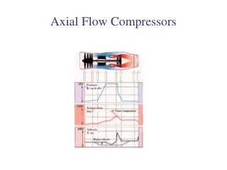
Chapter 5 Axial Flow Compressors • Subsonic compressors will be considered here as supersonic compressors have not proceeded beyond experimental stage. • A Comparison of • Axial Flow Compressors and Turbines • Turbine:- Accelerating flow - Successive pressure drops and consequent reductions in enthalpy being converted into kinetic energy • A1>A2 ⇨ converging passages Prof. Dr. O. Cahit ERALP
A Comparison ofAxial Flow Compressors and Turbines • Compressor :- Decelerating flow - Pressure rises are obtained through successive stages of diffusing passages with consequent reduction in velocity. • A1<A2 ⇨ diverging passages • Problems of compressors & turbines are different • in compressors - aerodynamic problems • in turbines - problems due to entry temperature and heat-transfer. • Boundary Layers - regions of low momentum air where viscous effects dominate over inertial effects. Prof. Dr. O. Cahit ERALP
A Comparison ofAxial Flow Compressors and Turbines • Boundary layers are far less happy in a compressive flow. BL in a compressor operate in an unfavourable pressure gradient [(+) 've ; p increase ] • BL in a turbine operate in a favourable pressure gradient[ (-)'ve ; p decrease. ] • This is the reason why a single stage turbine can create enough power to drive a number of stages of compressor. • Bend thin plates and stick them behind each other forming a stationary cascade of blades. • Let the flow be directed towards the inletofthis cascade of blades without any incidence. Prof. Dr. O. Cahit ERALP
A Comparison ofAxial Flow Compressors and Turbines • As A2 > A1 in subsonic flow (incompressible) • W2 < W1 & P2 > P1 • This is no more than a subsonic diffuser • To carry a mechanical load,some thickness is required. • If M < 0.3 incompressible • i.e. thus Prof. Dr. O. Cahit ERALP
A Comparison ofAxial Flow Compressors and Turbines • Clearly the outlet velocity W2 cannot decrease beyond a certain level (cannot be zero) (or W2≠ 0) • p W12 (since W2 is fixed by the lower limit) • One should design the compressor at the highest inlet velocity • But the losses ⇨Poα W12 • α 1/ p • Stage pressure ratio is limited and the number of stages are determined accordingly(single stage or multistage) Prof. Dr. O. Cahit ERALP
A Comparison ofAxial Flow Compressors and Turbines • Due to the contraction, the flow initially accelerates pressure drops (favourable to BL)( A1 > A1' ) • then • The amount of pressure rise between 1' to 2 is larger than that of 1 to 2. • i.e more diffusion the limit of Wmax is than of sonic limit. • More diffusion means less efficiency • i.e why we prefer compressor blades to be as thin as possible. Prof. Dr. O. Cahit ERALP
A Comparison ofAxial Flow Compressors and Turbines • The more the (camber), the more is the adverse pressure gradient, then seperation occurs earlier. • The seperated flow leaves the blade at an unwanted angle and unsteady situation. • All these problems in compressor cascades are due to Boundary layers. • Turbine problems are completely different since we want the pressure to drop along the flow direction. • The flow is a high "h" enthalpy or high temperature, high pressure (to low T low P) flow. Prof. Dr. O. Cahit ERALP
A Comparison ofAxial Flow Compressors and Turbines • The blades are such that minimum c/s area occurs at the trailing edge of the blades which is called the throat. • The flow area should contract continuously all the way along the blades in order not to have an adverse pressure gradient BL along the row. • Even an instantaneous discontinuity in the contraction of the passage results in a locally seperated BL, thus increased turbulence. • This might happen due to simplified manufacture for curvatures such as two circles. • This results in extremely high heat transfer coefficient, thus the blade will not last 10 minutes. Prof. Dr. O. Cahit ERALP
A Comparison ofAxial Flow Compressors and Turbines • For the Axial Compressors and turbines the basic components are rotors and stators, the former carrying the rotating blades and the latter the stationary rows which serve to recover the pressure rise from the kinetic energy imparted to the fluid by the rotor blades as in compressors and/or to redirect the flow into an angle suitable for entry to the next row of moving blades. • A compressor stage is composed of a rotor followed by a stator, where as a turbine stage is composed of a stator followed by a rotor . Prof. Dr. O. Cahit ERALP
A Comparison ofAxial Flow Compressors and Turbines • In Compressors • It is usual to provide a row of stator blades –Inlet Guide Vanes (IGV's) at the upstream of the first stage. These direct the axially approaching flow correctly into the first row of rotor blades. Thus deflect the flow from axial direction to off-axial direction. IGV's are turbine type of blades. • Two forms of rotor construction is used • Drum type-suitable for industrial applications • Disc type - suitable for aircraft applications low weight, high cost) Prof. Dr. O. Cahit ERALP
A Comparison ofAxial Flow Compressors and Turbines • Another important constructional detail is the contraction of the flow annulus from the low the high pressure end of the compressor. • This is necessary to maintain a reasonably constant axial velocity along. most compressors are designed on the basis of constant axial velocity because of the simplification in design procedure. One could have a rising hub or a falling shroud in compressors. Prof. Dr. O. Cahit ERALP
Elementary Theory For Axial Flow Compressors • Basic principle : Acceleration of the working fluid followed by diffusion to convert the acquired kinetic energy into a pressure rise. • The flow is considered as occuring in the tangential plane at the mean blade height where the blade peripheral velocity is u. • When the annulus is unrolled, since the blade C/S changes from Hub to Tip, one C/S is chosen • (e.g. at mid blade height) • and a series of constant C/S aerofoils result. • These are called a 2-D cascade of aerofoils. Prof. Dr. O. Cahit ERALP
Elementary Theory For Axial Flow Compressors • A semi- cascade can be produced if the cascade end boundary effects are eliminated (The flow in the channels are not aware of what happens at the ends) • The aerodynamics of a cascade repeats itself with a periodicity of s (pitch). • As the flow is going through the cascade, the end wall BL grows in thickness, thus the axial velocity grows. • To take care of this, BL is sucked; or a large "Aspect Ratio" cascade where the effect of end wall BL is less observed, is used. • v-absolute velocity • w-relative velocity • u- peripheral blade velocity Prof. Dr. O. Cahit ERALP
Elementary Theory For Axial Flow Compressors • On the rotor, turn your head into the wind, and the drought you feel is the relative velocity w • Connect the absolute velocity vectors (u and v) together arrow-head to arrow-head, the tails became the relative velocity vector (w) W2< W1P2 > P1 across the rotor • across the stator Prof. Dr. O. Cahit ERALP
Elementary Theory For Axial Flow Compressors • From the velocity triangles • U/Va= tan 1 + tan 1(5.1) • U/Va= tan 2 + tan 2(5.2) • The axial velocity Va is assumed to be constant throughout the stage. • The work absorbed by the stage, from the consideration of the"change of angular momentum", in terms of work done per unit mass flow rate or specific work input is: • (5.3 , 5.4) • or (5.5) Prof. Dr. O. Cahit ERALP
Vθ2 – Vθ1 α2 β1 inlet α1 β2 exit V2 V1 W2 Va Vθ1 U Vθ2 Elementary Theory For Axial Flow Compressors Combined Velocity Triangle for Axial Compressor Stage Prof. Dr. O. Cahit ERALP
Elementary Theory For Axial Flow Compressors • The input energy is absorbed usefully toincrease p and v and waste fully to increase T (frictional losses) • regardless of losses (efficiency)the whole input = Tos • If V1 = V3 • (5.6) • In actual fact the stage temperature rise will be less than this owing to 3D effects in the compressor annulus (growing end wall B/L) Prof. Dr. O. Cahit ERALP
Elementary Theory For Axial Flow Compressors • Analysis of experimental results has shown that it is necessary to multiply the results given by equation 5.6 by the so called work done factor which is a number < 1 • λ= Actual work absorbing capacity /Ideal work absorbing capacity • The explanation of this is based on the fact that the radial distribution of axial velocity is not constant across the annulus but becomes increasingly peaky as the flow proceeds as shown in the figure. • From eqn. 5.1 :Va tan 1 = U- Vatan 1 • Substitute into 5.5 : • since1& 1 are fixedwhile Va increase then w decrease Prof. Dr. O. Cahit ERALP
Va Va Va mean Va mean Elementary Theory For Axial Flow Compressors • From eqn. 5.1 :Va tan 1 = U- Vatan 1 • Substitute into 5.5 : • since1& 1 are fixedwhile Va increase then w decrease Prof. Dr. O. Cahit ERALP
Elementary Theory For Axial Flow Compressors • If the compressor has been designed for a constant radial distribution of Va, the effect of an increase in Va in the central region will be to reduce the work capacity of blading in that area. • This reduction however should be compensated by increases in the regions of the root and tip of the blading because of the reductions in Va at these parts of the annulus. Unfortunately this is not the case since; • Influence of BL's on the annulus walls • Blade tip clearances has an adverse effect on this compensation and the net result is a loss in total work capacity) • .W = Actual amount of work which can be supplied to the stage. Prof. Dr. O. Cahit ERALP
Elementary Theory For Axial Flow Compressors Prof. Dr. O. Cahit ERALP
Elementary Theory For Axial Flow Compressors • Actual stage temperature rise : • The pressure ratio: • s= stage isentropic efficiency Prof. Dr. O. Cahit ERALP
Degree of Reaction • =static pressure rise across the rotor/ • / static pressurerise across the whole stage • It is also a measure of how much of the total pressure rise across the stage occurs in the rotor. • Since Cp doesn't vary much across a stage, will be equal to the corresponding temperature rises. Prof. Dr. O. Cahit ERALP
Degree of Reaction • TR = Temperature rise across the rotor • TST = Temperature rise across the stator • TS = Stage temp. Rise • Assuming =1.0 Prof. Dr. O. Cahit ERALP
Degree of Reaction • The steady flow energy eqn : • with eqn (5.8) : • But • since Prof. Dr. O. Cahit ERALP
Degree of Reaction • (5.9) Prof. Dr. O. Cahit ERALP
Degree of Reaction • For 50% reaction which is a wide practice (=0.50) • from equations 5.1& 5.2 • ⇨1=2 , 2=1 • since V1=V31=3 (for repeating stages) • For ⇨ symmetrical blading • 1=2=3 , 1=2 Prof. Dr. O. Cahit ERALP
Degree of Reaction • Eqn 5.9 is derived for =1 • Actually will differ from 50% slightly because of the influence of ; • but still will be called symmetrical blading. Prof. Dr. O. Cahit ERALP
3D Flow • Up to here the analysis has been confined to a 2D flow basis at one particular radial position in the annulus ; which is usually chosen to be "at the mean blade height" Before considering its extension to cover the whole blade height , attention must be given to some basic principles of 3D flow. • For high H/T ratio 2D assumption is reasonable • Low H/T ratio Radial flow components should be considered. Prof. Dr. O. Cahit ERALP
3D Flow • Assumption • Any radial flow within the annulus occurs only while the fluid is passing through the blade rows. The flow in the gaps between successive blade rows will be in Radial Equilibrium. • Basic Assumption Vr =0 at the entry and exit of a blade row. • A commonly used design method is based on this principle and an equation is set up to fulfill the requirement that radial pressure forces must act on the air elements in order to provide the necessary radial acceleration associated with the peripheral velocity component V. Prof. Dr. O. Cahit ERALP
p+dp dr Vθ p+dp/2 p+dp/2 p r dθ 3D Flow Prof. Dr. O. Cahit ERALP
3D Flow • From the figure the force balance in radial direction i.e pressure forces = centrifugal forces Vr =0 • Here for small • Cancelling dq through the eqn and neglecting 2nd orderterms such as dpdr. • (Radial Equilibrium Condition) Prof. Dr. O. Cahit ERALP
Radial Equilibrium Condition • The Radial equilibrium equation may be used: • to determine Va (r) once V(r) is chosen(design orindirect problem) • to determine Va (r), V (r) produced by a selected blade shape i.e. a (r) (Direct problem) • The stagnation enthalpy "h0" at any radius r • since Prof. Dr. O. Cahit ERALP
Radial Equilibrium Condition • Differentiating wrt. r we have • Lets assume that the change in pressure across the annulus is small and the isentropic relation can be used. • i.e =const. is valid with little error. • In differential form OR • substituting into the previous relation; Prof. Dr. O. Cahit ERALP
Radial Equilibrium Condition • Introducing the Radial Equilibrium condition • Apart from the regions near the walls of the annulus the stagnation enthalpy (and To) is uniform across the annulus at the entry to the blade rows. • Thus • in any plane between a pair of blade rows. Prof. Dr. O. Cahit ERALP
Radial Equilibrium Condition • A special case may now be considered in whichVa=const. is maintained across the annulus, so that • OR • Integrating this gives:OR • Thus the whirl velocity component of the flow varies inversely with the radius. • This is the Free Vortex condition. Prof. Dr. O. Cahit ERALP
Radial Equilibrium Condition • The Free Vortex Radial Equilibrium is Satisfied by: • Constant specific work input dho/dr = 0 • Constant axial velocity at all radii i.e. dVa/dr =0 • Free Vortex variation of whirl velocity (Vr =const) Prof. Dr. O. Cahit ERALP
Radial Equilibrium Condition • There is no reason why the specific work input should not • be varied with radius i.e. .It would then be • necessaryto choose a radial variation of one of the other variables say Va (r) and determine the variation of V with r to satisfy the radial equilibrium. Thus in general a design can be based on arbitrarily choosen radial distributions of any two variables and the appropriate variation of the third can be determined by using the equation • Note:or any other variable may be used instead of Prof. Dr. O. Cahit ERALP
Blade Design • Having determined the air angle distributions to give the required stage work it is now necessary to convert these into blade angle distributions from which the correct geometry of the blade forms may be determined. • Air Angles Blade angles Blade Geometry • The common practice is to use the results of the wind tunnel tests to determine the blade shapes to give the required air angles. The aim of the cascade testing is to determine the required angles for • Maximum mean deflection • Minimum mean total head loss. Prof. Dr. O. Cahit ERALP
Blade Design • β1v,α1v = Blade inlet angle • β2v,α2v = Blade outlet angle • β1, α1 = Air inlet angle • β2, α2 = Air outlet angle • W1,V1 = Air inlet velocity • W2,V2 = Air outlet velocity • s = pitch • c = chord • θ = camber = α1v – α2v • ξ = stagger = 0.5(α1v + α2v) • є = deflection = α1 – α2 • i = incidence = α1 - α1v • δ = deviation = α2 – α2v Prof. Dr. O. Cahit ERALP
Blade Design Prof. Dr. O. Cahit ERALP
Blade Design • The loss in non-dimensional form w = • It is desirable to avoid numbers with common multiples for the blades in successive rows to reduce the likelihood of introducing resonant frequencies. • The common practice is to choose an even number for the stator blades and a prime number for the rotor blades. • The bladeoutlet angle “2v”can not be determined from the air outlet angle “2” until the deviation angle “”has been determined. Prof. Dr. O. Cahit ERALP
Design Procedure β2 β1 know how ≈ 3 ε = β1 – β2 h/c h ε* β2 α2 c s/c Des. Defl. Curve rm s n = 2πrm/s number of blades n ns even nr prime recalculate s/c , h/c Blade Design Prof. Dr. O. Cahit ERALP
Blade Design • Ideally the mean direction of the air leaving the cascade would be that of the outlet angle is of the blades. • But in practice it is found that there is a deviation which is due to the reluctance of the air to turn through the full angle required by the shape of the blade. • Empirical equations are employed to estimate . • where : • where "a" = the distance to the point of maximum camber from the leading edge. • If the camber arc is circular (2a/c) =1 Prof. Dr. O. Cahit ERALP
Blade Design • Using the values of “c, 1v, 2v, “; it is possible to construct the circular arc camberline of the blade around which an aerofoil section can be built up. • This method can now be applied to a selected number of points along the blade length to get a complete picture of the blade form. Prof. Dr. O. Cahit ERALP
Calculation ofStage Performance • After the completion of stage design it will now be necessary to check over the performance, particularly in regard to the efficiency which for a given work input will completely govern the final pressure ratio. • This efficiency is dependent of the total pressure drop for each of the blade rows comprising the stage and in order to evaluate these quantities it will be necessary to revert the loss measurements in cascade tests. • Lift and profile drag coefficients CL and CDP can be obtained from measured values of mean loss w. Prof. Dr. O. Cahit ERALP
Calculation ofStage Performance • The static pressure rise across the blades is given by (incompressible assumption) Prof. Dr. O. Cahit ERALP