Measures of Central Tendency

1. Measures of Central Tendency

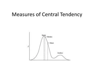
2. Measures of Central Tendency • These measures indicate a value, which all the observations tend to have, or a value where all the observations can be assumed to be located or concentrated • There are three such measures: i) Mean ii) Median, Quartiles, Percentiles and Deciles iii) Mode

3. Mean • Arithmetic Mean • Harmonic Mean • Geometric Mean 1) Ungrouped data Sum of Observations x1 + x2 +….x n Mean = ----------------------------- = -------------------- Number of Observations n

4. 2) Grouped data When the data is grouped, prepare frequency table Class IntervalMid-point of ClassFrequency ( fi ) Interval ( Xi ) -- x 1 f 1 -- -- -- -- x k f k ∑ f i x i x = --------------- ∑ f i Where xi is the middle point of the ith class interval. f i is the frequency of the ith class interval. fi xi is the product of fi and xi and k is the number of class intervals

5. Median • Whenever there are some extreme values in data, calculation of A.M. is not desirable • Median of a set of values is defined as the middle most value of a series of values arranged in ascending / descending order • If the number of observations is odd, the value corresponding to the middle most values is the median • If the number of observations is even then the average of the two middle most values is the median

6. Example 3144 4784 4923 5034 5424 5561 6505 6707 6874 4187 4310 4506 4745 5071 2717 2796 3144 3527 3098 3534 Ascending Order 2717 2796 3098 3144 3527 3534 3862 4187 4310 4506 4745 4784 4923 5034 5071 5424 5561 6505 6707 6874 Hence, the number of observations is 20, and therefore there is no middle observation. Two middle most observations 10th and 11th . 4506 + 4745 9251 Median = -------------------- = --------- = 4625.5 2 2

7. Quartiles • Median divides the data into two parts such that 50 % of the observations are less than it and 50 % are more than it. • Similarly there are “Quartiles”. There are three quartiles viz. Q1, Q2 and Q3. These are referred to as first, second and third quartiles. • The first quartile Q1, divides the data into two parts such that 25 % of the observations are less than it and 75 % more than it. • The second quartile Q2 is the same as median. • The third quartile divides the data into two parts such that 75 % observations are less than it and 25 % are more than it.

8. Percentiles • Percentiles splits the data into several parts, expressed in percentage. • A percentage is also known as centile, divides the data in such a way that “given percent of the observations are less than it. • For example, 95 % of the observations are less than the 95th percentile • It may be noted that the 50th percentile denoted as P50 is the same as the median

9. Deciles • The deciles divides the data into ten parts • First decile (10%) • Second (20%) and so on

10. Mode • It is defined in such a way that it represents the fashion of the observations in a data. • Mode is defined as the most fashionable value, which, maximum number of observations have or tend to have as compared to any other value. • Observations are 2, 4, 4, 6, 8, 8, 8, 10, 12 Here mode is 8 because 3 observations have this value.

11. Measures of Variation/ Dispersion • Measures of variation/dispersion provide an idea of the extent of variation present among the observations These are- i) Range ii) Mean Deviation iii) Standard Deviation iv) Coefficient of Variation

12. Range • It is the simplest measure of variation, and is defined as the difference between the maximum and the minimum values of the observations Range = Maximum Value – Minimum Value Since the range depends only on the two viz. the minimum and the maximum values, and does not utilize the full information in the given data, it is not considered very reliable or efficient.. • Coefficient of scatter is another based on the range of the data Range Maximum – Minimum -------------------- = ------------------------------ Maximum + Minimum Maximum + Minimum It gives an indication about variability in the data

13. Mean Deviation • In order to study the variation in a data, one method could be to take into consideration the deviation of all the observation from their mean • Example ( Mean 50) Observation Deviation from Mean 50 0 49 - 1 51 +2 40 -10 10 -40 90 +40

14. Mean Deviation for Ungrouped Data • If the data is ungrouped and the observations for certain variable x, are x1, x2, x3, ….., xn ∑ xi - x Mean Deviation = --------------- n For the data comprising observations 1,2,3, it can be calculated as follows (xi) xi – x xi – x 1 -1 1 2 0 0 3 +1 1 --------------------------------------- Sum 6 0 2 Mean 2 0 2 / 3 Thus the mean deviation is 2 / 3 = 0.67

15. Mean Deviation for Grouped Data

16. ∑ ƒί│x i - x│ 19300 Mean Deviation = --------------- = -------- = 965 ∑ ƒί 20 x i is the middle point of class interval x is the mean ƒί is the frequency of the i th class interval

17. Variance and Standard Deviation • While calculating mean deviation, the absolute values of observations from the mean were taken because without doing so, the total deviation was zero for the data comprising values 1,2 and 3 even though there was variation present among these observations. • However another way of getting over this problem of total deviation being zero is to take the squares of deviations of the observations from the mean xi xi -x ( xi -x )2 1 -1 1 2 0 0 3 +1 1 -------------------------------------------------- Sum 6 0 2 Mean 2 0 2/3 (=0.67)

18. Calculation of variance and standard deviation for ungrouped data 1 Variance (σ2 )= ---- ∑ ( xi -x )2 n 1 = ----- x (2) = 0.67 3 The square root of σ2 i. e σ is known as the standard deviation Standard Deviation (σ ) =0.67 = 0.82

19. Calculation of Variance and Standard Deviation for Grouped Data

20. S.D. = Variance = 1447500 = 1203.12

21. Combining Variances of Two Populations • The mean and S.D. of the “lives” of tyres manufactured by two factories of the “Durable” tyre company, making 50,000 tyres, annually, at each of the two factories, are given below. Calculate the mean and standard deviation of all the 100000 tyres producced in a year. Group Mean (‘000 kms.) S.D. (‘000 kms.) 1 60 8 2 55 7

22. We know that if there is one set of data having n1 observations with mean=m1 and s.d.= σ1and another set of data havingn2 observations with mean = m2 and s.d. = σ2 then the mean (m) and variance (σ2) of the combined data with (n1 + n2) observations are given as m = n1m1 + n2m2 / n1 + n2 σ2 = n1(σ12 + d12) +n2 (σ22 +d22 ) / n1 +n2 d1 = m1 – m d2 = m2 – m m= combined mean of both the sets of data

23. Factory 1 : n1 = 50, m1 = 60 and σ1= 8 Factory 2 : n2 = 50, m2= 55 and σ1= 7 Substituting these values in the above formulas Mean = (50 x 60) + (50 x 55) / (50+50) = (3000 + 2750) / 100 = 5750 / 100 = 57.5 Thus the mean life of the tyres manufactured by the company is 57,500 kms.

24. Therefore, d1 = m1 – m = 60 - 57.5 = 2.5 d2 = m2 – m = 55 - 57.5 = -2.5 50x ( 82 + 2.52) + 50 x (72 + 2.52) Variance (σ2)= __________________________ 50 + 50 = (50x70.25) +(50x 55.25) / 100 = 3512.5 + 2762.5 /100 = 6275 /100 = 62.75

25. Variance = (σ2)= 62.75 Therefore S.D. (σ) = 62.75 = 7.92 Thus, the S.D of the lives of tyres produced by the company is 7,920 kms.

26. Mean Deviation The mean deviation is defined as ∑ ƒί xi - x Mean Deviation = ------------------- ∑ ƒί Where, x1 is the middle point of i th class interval ƒίis the frequency of the ith class interval and x Is the arithmetic mean of the I.Q. scores

28. From this data, we get ∑ ƒίxi 7150 Mean = ----------- = ---------- = 71.5 ∑ ƒί100 ∑ ƒί xi - x 1450 Mean Deviation = ------------------- = --------- = 14.5 ∑ ƒί 100 Thus the average score is 71.5 and the mean deviation of the score is 14.5

29. Suppose we are required to calculate only standard deviation for the above data, then the table is constructed as below

30. ∑ ƒίxi 7150 Mean = ----------- = ---------- = 71.5 ∑ ƒί100 ∑ ƒίxi 2__ (∑ ƒί)_ (x_)2 538500 – 100 (71.5)2 S.D. = ----------------------------- = -------------------- ∑ ƒί100 = 272.75 = 16.5 Thus, the s.d. of the I.Q. scores is 16.5

31. Coefficient of Variation • It is a relative measure of dispersion that enables us to compare two distributions. • It relates the standard deviation and the mean by expressing the standard deviation as a percentage of the mean σ • C. V. = --------- x 100 x

32. Example • For the data 103,50,68,110,105,108,174,103,150,200,225,350,103 find the range, Coefficient of Range and coefficient of quartile deviation 1) Range = H –L = 350 - 50 =300 H – L 300 2) Coefficient of range = ----------- = ---------- = 0.7 H + L 350+50

33. To find Q1 and Q3 we arrange the data in ascending order n+1 14 ------- = ------ = 3.5 4 4 3 (n+1) ----------- = 10.5 4 Q1 = 103 + 0.5 103-103) = 103 Q2 = 174 + 0.5 (200 – 174) = 187

34. Q3 – Q1 187 - 103 Coefficient of QD = ------------- = ------------ = 0.2896 Q3 + Q1 187+103

35. Example • A purchasing agent obtained a sample of incandescent lamps from two suppliers. He had the sample tested in his laboratory for length of life with the following results. Length of lightSample ASample B in hours 700 – 900 10 3 900 – 1100 16 42 1100 - 1300 26 12 1300 – 1500 8 3 Which company’s lamps are more uniform?

36. Sample A

37. 32 u A = -------- = 0.533 60 x A = 1000 + 200 u = 1000 + 200 (0.533) = 1106.67 1 68 σ2u = ---- ∑ f u2 - (u )2 = ------- - (0.533)2 N 60 σ2u = 1.133 – 0.2809 = 0.8524 σ x = 200 x 0.9233 = 184.66 C. V. for sample A = σ A / x A x 100 = 184.66 / 1106.67 x 100 = 16.68 %

38. Sample 2