Download
1 / 20
200 likes | 319 Views
MACROECONOMICS. Chapter 8 Economic Growth II: Technology, Empirics, and Policy. Outline of the Chapter. Including technological change into Solow Model. Testing the model with data. Discussing policy options to improve the standard of living. New growth theories.

E N D
MACROECONOMICS Chapter 8 Economic Growth II: Technology, Empirics, and Policy
Outline of the Chapter • Including technological change into Solow Model. • Testing the model with data. • Discussing policy options to improve the standard of living. • New growth theories.
Including Technological Progress • Suppose technology is labor-augmenting. • It increases efficiency of labor. • It increases the “effective” number of workers. • Y = F(K,LE) • Example • Y = Kα(LE)1-α • y = kα where y = Y/LE and k = K/LE
What Does E Include? • Knowledge • Health • Education • Institutions that promote growth of production
Long Term Growth of E • If efficiency of labor (E) doubles in 35 years, E must be growing at annual rates of 2%. • If E doubles in 10 years, annual growth rate is 7%. • The growth rate of E, labeled g, will be given outside of the system (exogenous) in our analysis.
Long Term Growth of LE • If E grows at rate g and population grows at rate n, then LE must grow at rate g+n. • %Δ(LE) = %ΔL + %ΔE • If LE grows by n+g, then, once the economy reaches the steady state (k*), K must also grow by n+g to keep it at that level.
Steady State • Steady State k was the level of k, once reached, remained there. • No increase or decrease of k takes place once that equilibrium (k=k*) is reached. • Accumulation of k depends on investments being larger than the depreciation plus n+g. • sf(k*) = (δ+n+g)k* • If savings (=investments) are larger than (δ+n+g)k, k will increase; smaller: decrease.
Steady State and Golden Rule y y= (Y/LE) (δ+n+g)k sy k = (K/LE) k k k*
Steady State and Golden Rule y y= (Y/LE) (δ+n+g)k sy c* s*y k = (K/LE) k*
Growth Rates in Steady State • In steady state, k=k* and y=y*. • k=K/LE implies that at steady state, in order to keep k constant, K must increase at rate n+g while k (capital per effective worker) remains constant. • y=Y/LE implies that to keep y=y*, Y must grow at rate n+g. • Per capita income must grow at g; capital-output ratio constant.
Steady State and Golden Rule • Steady State: • sf(k*)=(δ+n+g)k* • f(k*)-c*=sf(k*) • c*=f(k*)-(δ+n+g)k* • But, the slope of f(k) at Golden Rule is (δ+n+g) which is the definition of MPK. • If the economy is at Golden Rule Steady State, then MPK (=real rental price of capital) must be equal to δ+n+g.
Steady State • If long run growth of real GDP is 4% with population growth of 1% and technology growth of 3%, then we fulfill the requirements of steady state. • If Y grows at 8% with 2% population growth and 3% technology growth we are not at steady state. (See slide #8)
Further Implications • Constant returns to scale yields: • L(MPL)+K(MPK)=Y • Y growth is n+g • L growth is n • K growth is n+g • MPL growth must be g and MPK growth must be zero. • US data show g=2% with MPL growth 2% and MPK constant!
Is U.S. at Golden Rule? Given n = 0.01 g = 0.02 δk = 0.1y k = 2.5y MPK(k) = 0.3y MPK will become smaller as k increases. In order for k* to be a higher number, s has to increase.
Endogenous Growth Models • Knowledge does not have diminishing returns, and it has positive externalities. • Once included in the production function, it eliminates the k* steady-state property. • Production function can be straight line (Y=AK) or increasing slope (as E grows fast in Y=F[K,(1-u)LE]).
Endogenous Growth Models As long as capital accumulation takes place, there is no end to growth of income.
Convergence or Divergence • Same production function, same s, g, n, δ. • Convergence, even if they start at different k. • Production function might be connected to urbanization. • Same production function, different s, g, n, δ. • Divergence • Different production functions: divergence
Similarities • Production efficiency (E) and factor accumulation (LE) and K seem to correlate (go hand in hand). • Maybe an efficient economy promotes capital accumulation. • Maybe there are positive externalities to capital: more savings, better production function. • Maybe better institutions and policies affect both.
The economy can grow faster than normal for a period until it reaches the point where it would have been without the crisis, when it reaches its full potential again. (Friedman) If the shortfall in demand persists it can do lasting damage to supply, reducing the level of potential output (scenario 2) or even its rate of growth (scenario 3). If so, the economy will never recoup its losses, even after spending picks up again. In a recession firms shed labor and mothball capital. If workers are left on the shelf too long, their skills will atrophy and their ties to the world of work will weaken. When spending revives, the recovery will leave them behind. Output per worker may get back to normal, but the rate of employment will not. http://www.economist.com/specialreports/displayStory.cfm?story_id=14530093 World Economic Outlook: cost of 88 banking crises over the past four decades. On average, seven years after a bust an economy’s level of output was almost 10% below where it would have been without the crisis.
Does Free Trade Promote Growth? • Compare countries ranked according to openness with growth. • Study the impact of openness on growth. • Instead of trade, look at geography. It is an instrumental variable that correlates with trade but does not correlate with other variables that enhance growth.