Download
1 / 59
590 likes | 693 Views
Delayed Congestion Response Protocols Thesis By Sumitha Bhandarkar Under the Guidance of Dr. A. L. N. Reddy. Layout of the presentation Introduction to “TCP-Friendliness” Motivation for Delayed Congestion Response Protocols Delayed Congestion Response Protocols

E N D
Delayed Congestion Response Protocols Thesis By Sumitha BhandarkarUnder the Guidance of Dr. A. L. N. Reddy
Layout of the presentation • Introduction to “TCP-Friendliness” • Motivation for Delayed Congestion Response Protocols • Delayed Congestion Response Protocols • Conclusions And Future Work • Related Work
Introduction to “TCP-Friendliness” • Stability of internet depends on protocols that respond to congestion • Congestion Control Algorithm of TCP results in drastic changes in sending rate • When used with real-time audio/video application, this will cause drastic changes in user perceived quality • UDP looks like a good alternative for such applications
Introduction to “TCP-Friendliness” (contd.) • Extensive use of UDP could result in • Extreme unfairness to existing TCP applications • Congestion collapse of the internet • Lot of interest in new class of protocols called “TCP-Friendly” Protocols • “TCP-Friendliness” indicates that the protocol chooses to send at a rate no higher than TCP under similar conditions of round trip delays and packet losses
Introduction to “TCP-Friendliness” (contd.) An analytical model for TCP was developed by J. Padhye et. al. which shows - T = S R 2p/3 + TRTO (3 3p/8) p ( 1 + 32p2) T : Throughput S : Packet Size R : Round Trip Time TRTO : Retransmission Timeout p : Loss Rate
Introduction to “TCP-Friendliness” (contd.) • Simplified Throughput Equation • 3/2 T = R * p • In a very general sense a protocol which maintain the sending rate to at most some constant over the square root of the packet loss rate is said to be “TCP-friendly”.
Motivation For Delayed Congestion Response Protocols • Congestion in the network is notified to the protocol, in most cases, through packet drops. • TCP as well as most of the TCP-friendly protocols reduce the sending rate once and as soon as allowed by protocol design, when a packet drop is noticed. • By delaying congestion response by ‘’ RTTs, the transport protocol can provide application with an early warning regarding an impending reduction in sending rate.
Motivation For Delayed Congestion Response Protocols (contd.) • Smart applications can be designed to combine Early Notification with buffering techniques to provide smooth output. • For applications that cannot take advantage of early notification, smooth sending rate can be provided by reducing the congestion window smoothly, during the period ‘’ after a packet drop. • By studying the time scales over which we can delay the congestion response insight can be gained regarding the time scales for defining “TCP-Friendliness”.
Delayed Congestion Response Protocols • Protocols where response to congestion is deliberately delayed by ‘’ RTTs when a congestion is notified. • Congestion control dynamics characterized by (f1(t), f2(t), , ). f2(t) Pkt Drop C w n d f1(t) Time
DCR-I • f2(t) is an increasing function • For simplicity of implementation and analysis we set • f1(t) as an additive function. • f2(t) = f1(t). Pkt Drop f2(t) f1(t) C w n d Time
DCR-I • Thus we have, • f1(t) : wt+R wt + ; > 0 • f2(t) : wt+R wt + ; > 0 , tdrop < t < tdrop + • wtdrop + * wtdrop + - ; < 1 • wt is the congestion window at time t • R is the RTT • , and are constants
DCR-I Steady State Analysis f2(t) Pkt Drop C w n d f1(t) A t1 t2+ t2 Time Throughput = Number of packets between two successive drops Time between two successive drops
DCR-I Steady State Analysis (contd.) ( /2 ) ( 1 + ) / ( 1 - ) = R p Comparing with the TCP-equation, the condition of TCP-Friendliness is : 3 ( 1 - ) = ( 1 + )Infinite number of values can be chosen for and that satisfy the above condition . We chose = 1 and = 1/2 since it is makes DCR-I very similar to TCP-reno.
DCR-I • Implementation • Testing platform was ns-2 • Modifications were made to the existing TCP-reno. • When congestion in the network was notified, the time-to-response was noted. • Congestion window was continuously increased until the time-to-response, at which time it was cut down by half.
DCR-D • Primary aim of DCR-D is to provide smooth response. • f2(t) is thus chosen to be a decreasing function and is set to1. Pkt Drop f1(t) C w n d f2(t) Time
DCR-D • We have, • f1(t) : wt+R wt + ; > 0 • f2(t) : wt+R * wt ;0 < < 1, tdrop < t <tdrop + • wt is the congestion window at time t • R is the RTT • , and are constants
DCR-D Steady State Analysis Pkt Drop f2(t) C w n d f1(t) N1 N2 t1 t2+ t2 Time Throughput = Number of packets between two successive drops Time between two successive drops
DCR-D • Steady State Analysis (contd.) • Set K = , the factor by which the congestion window is decreased over the period of ‘’ RTTs • 1 • = R (2p(1-K)/(1+K) + p ([2(1-K)/lnK(1+K)] + 1)) • The above equation is TCP-Friendly if second term in the denominator is negligible
DCR-D • Steady State Analysis (contd.) • Condition for TCP-Friendliness is : • p2 . (1-K) + 1 = 0 lnK (1+K) • For different values of K, the results of the above equation is given as follows -
DCR-D • Steady State Analysis (contd.) • With K = 0.8, the throughput equation can be written as1 • = R (2p(1-K)/(1+K) + 0.0041* p) • Second term in the denominator is negligible. • Comparing the above equation with TCP equation we have, • 3 ( 1-K) = (1+K) • With K = 0.8, = 0.333
DCR-D • Implementation • Testing platform was ns-2 with modifications made to the existing TCP-reno. • Two modes of operation • Increase mode : seeking bandwidth using f1(t) • Decrease mode : reducing bandwidth using f2(t) • On congestion notification start a delay timer for ‘’ RTTs and get into decrease mode. • When the delay timer expires return to Increase mode.
DCR-D • Implementation(contd.) • While entering the decrease mode note down the target value of the congestion window to be achieved at the end of decrease mode. • If packet is dropped in decrease mode, • Reset the delay timer. • Reduce the congestion window to its target value drastically. • Set a new delay timer to take care of latest congestion. • Note down the current target value. • Reasoning: Packet drop during decrease mode indicates high level of congestion. Thus drastic reduction in congestion window is required as compared to the smooth reduction using f2(t) .
DCR-D Congestion Window Evolution at High Droprates Pkt Drop Pkt Drop C w n d TargetValue Original Timer Time NewTimer
DCR-C • f2(t) is an constant function Pkt Drop f2(t) C w n d f1(t) Time
DCR-C • We have, • f1(t) : wt+R wt + ; > 0 • f2(t) : wt+R wt ; tdrop < t <tdrop + • wtdrop + * wtdrop + - ; < 1 • wt is the congestion window at time t • R is the RTT • , and are constants • Analysis shows this protocol cannot be TCP-Friendly. So simulations were not conducted for this protocol.
Simulation Topology Src 1 Sink 1 Src 2 Sink 2 ..... ..... B MbpsD ms R1 R2 Bottleneck Link Sink n Src n
Simulation ResultsDCR-I Fairness Index at Different Droprates
Simulation Results DCR-I Fairness Index at Different Buffer Sizes
SimulationResultsDCR-I Fairness Index with mixed workload
Simulation Results DCR-I Sample per-flow droprates for mixed workload
Simulation Results DCR-I Fairness Index at Different Droprates with Drop Tail Router
Simulation Results DCR-I Sample values of per-flow droprates (Drop Tail Router)
Simulation ResultsDCR-I Effects of Clock Resolution
SimulationResultsDCR-D Fairness Index at Different Droprates
SimulationResults DCR-D Fairness Index at Different Buffer Sizes
SimulationResultsDCR-D Fairness Index with mixed workload
Simulation Results DCR-D Sample per-flow droprates for mixed workload
Simulation Results DCR-D Fairness Index at Different Droprates with Drop Tail Router
Simulation Results DCR-D Sample values of per-flow droprates (Drop Tail Router)
Simulation Results DCR-D Effects of Clock Resolution
Simulation Results DCR-D Effects of Clock Resolution With Compensated
Simulation Results Measure of smoothness • Protocols used with real-time audio-video application require smooth sending rates • Use coefficient of variance as a measure of smoothness • Note throughput at intervals of time • For each flow compute the cov as (standard deviation) / (mean) of these values • For the protocol, the cov is the average cov of all the flows using that protocol.
Simulation Results DCR-D Coefficient of Variance at Different Droprates ( = 0.5s)
Simulation ResultsDCR-DCoefficient of Variance at Different values of (p = 0.1%)
Conclusions • In this thesis, we have, • provided the general frame work for Delayed Congestion Response protocols. • examined three cases in particular and shown through analysis and simulations that two of these can be TCP-friendly for a wide range of network parameters. • Using DCR-D, shown that sending rate can be made smoother through the proper design of the function f2(t).
Conclusions (contd.) • Regarding the TCP-Friendliness we have shown, • 1/ p is necessary but not sufficient condition for determining TCP-Friendliness. • TCP-Friendliness depends on the underlying buffer management scheme. • TCP-Friendliness is affected by the type of workload on the system, even in the presence of an active buffer management scheme.
Future Work • Work needs to be done in synthesizing the general equations to provide proper guidelines for choosing the values of (f1(t), f2(t),, ). • Substantial work needs to be still done to characterize TCP-Friendliness
Related Work • “ModelingTCP Throughput: A simple Model and its Empirical Validation” by J.Padhye, V. Firoiu, D.Towsley and J.Kurose. • Developed an Analytical Model for TCP’s congestion control mechanism in terms of loss rate and RTT • Captures the behavior of fast retransmit and the timeout mechanism. • Evaluated using network traces obtained from the internet.
Related Work (contd.) • “Equation-Based Congestion Control for Unicast Applications”by Sally Floyd, Mark Handley, Jitendra Padhye, and Joerg Widmer. • Directly based on the TCP control Equation. • Receiver provides feed back for RTT calculations. • Receiver calculates loss event rate and feeds it back to sender. • Sender takes care of RTT calculations, retransmission ( if required) and adapts the sending rate based on the equation.