Download
1 / 19
190 likes | 336 Views
Verification of the Design of the Beam-based Controller. Jürgen Pfingstner 2. June 2009. Content. Analysis of the contoller with standard control engineering techniques Uncertanty studies of the response matix and the according control performance.

E N D
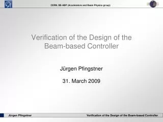
Verification of the Design of the Beam-based Controller Jürgen Pfingstner 2. June 2009
Content • Analysis of the contoller with standard control engineering techniques • Uncertanty studies of the response matix and the according control performance
Analysis of the contoller with standard control engineering techniques • Daniel developed a controller, with common sense and feeling for the system • I tried to verify this intuitive design with, more abstract and standardized methods: • Standard nomenclature • z – transformation • Time-discrete transfer functions • Pole-zero plots
The model of the accelerator 1.) Perfect aligned beam line • a.) 2 times xi -> 2 times amplitude • -> 2 times yj • b.) xi and xj are independent • Linear system without ‘memory’ Laser-straight beam QPi BPMi 2.) One misaligned QP Betatron- oscillation (given by the beta function of the lattice) y … vector of BPM readings x … vector of the QP displacements R … response matrix xi xj(=0) yi yj
Mathematical model of the controlled system ni ui ui+1 G(z) z-1 vi C(z) xi+1 yi xi ri z-1 (R*)-1 + R + + + - ui, ui+1 … controller state variables xi, xi+1 … plant state variables (QP position) C(z) … Controller G(z) … Plant ri … set value (0) … BPM measurements yi … real beam position vi … ground motion ni … BPM noise
System elements(SISO analogon!) • I controller • simple • allpass • non minimum phase Be aware about the mathematical not correct writing of the TF (matrix instead of scalar)
Stability and Performance • Stability • necessary attenuation at high frequencies • all poles at zero • Performance of the interesting transfer functions
Important transfer functions (set point following and measurement noise) (ground motion behavior)
Conclusions • Controller is: • very stable and robust (all poles at zero) • integrating behavior (errors will die out) • good general performance • simple (in most cases a good sign for robustness) • measurement noise has a strong influence on the output Further work • H∞ optimal control design
Uncertanty studies of the response matix and the according control performance Controller is robust, but is it robust enough? yes no done • Plan A: • Use methods from robust control to adjust the controller to the properties of the uncertainties (e.g. pole shift) • Plan B: • Use adaptive control techniques to estimate R first and than control accordingly • Answer to that question by simulations in PLACET
Tests in PLACET • Script in PLACET where the following disturbances can be switched on and off: • Initial energy Einit • Energy spread ΔE • QP gradient jitter and systematic errors • Acceleration gradient and phase jitter • BPM noise and failures • Corrector errors • Ground motion • Additional PLACET function PhaseAdvance • 2 Test series (Robustness according to machine drift): • Robustness regarding to machine imperfection with perfect controller model • Robustness regarding to controller model imperfections with perfect machine • Analysis of the controller performance and the resulting R
Test procedure • 1.) Misalign the QP at the begin of the simulation to create an emittance growth at the end of the CLIC main linac • 2.) Observe the feedback action in respect to the resulting emittance over time • 3.) Change certain accelerator parameter and repeat 1 and 2. • => The test focus on the stability and convergence speed more than on the steady-state emittance growth and growth rate. (see metric)
Performance metric Normalized emittance Allowed range for is where … Emittance produced by the DR and RTML … Emittance at the end of the main linac Theoretical minimum for
Results *1 … Values are according to the multi-pulse projected emittance *2 … Failed BPMs that deliver zeros are worse then the one giving random values.
Conclusions • Controller is very robust in respect to stability • It is sufficient in respect to disturbances
z – Transformation • Method to solve recursive equations • Equivalent to the Laplace – transformation for time-discrete, linear systems • Allows frequency domain analysis z – transfer function G(z) Discrete Bode plot Discrete System
Measures for the performance • Goal: Find properties of Rdist that correspond with the controller performance evnorm … eigenvalue norm L … matrix that determines the poles of the control loop Rdist … disturbed matrix Rnom … nominal matrix absnorm … absolut matrix norm
Information from absnorm and evnorm • evnorm absnorm • Controller works well for: • absnorm = 0.0 – 0.4 • Controller works well for: • evnorm = 0.5 – 1.0