Download
1 / 27
270 likes | 391 Views
How do ideas from perceptual organization relate to natural scenes?. Brunswik & Kamiya 1953. Thesis : Gestalt rules reflect the structure of the natural world Attempted to validate the grouping rule of proximity of similars Brunswik was ahead of his time… we now have the tools.

E N D
How do ideas from perceptual organization relate to natural scenes?
Brunswik & Kamiya 1953 • Thesis: Gestalt rules reflect the structure of the natural world • Attempted to validate the grouping rule of proximity of similars • Brunswik was ahead of his time… we now have the tools. Egon Brunswik (1903-1955)
Ecological Statistics of Perceptual Organization • Can we define these cues for real images? • Are these cues “ecologically valid”? • How informative are different cues? Figure/Ground Grouping
Task: detect generic pattern or group • Signal: class of patterns, known null hypothesis • Cues: optimal test is usually obvious • Result: mathematically precise characterization of when detection is possible • Task: capture “useful” information about the scene • Signal: natural image statistics, clutter • Cues: something computable from real pixels • Result: empirical statistics about relative power of different cues
distance [proximity] • region cues [similarity] • boundary cues [connectedness, closure, convexity] Cues: What image measurements allow us to gauge the probability that pixels i and j belong to the same group?
Learning Pairwise Affinities Sij – indicator variable as to whether pixels i and j were marked as belonging to the same group by human subjects. Wij – our estimate of the likelihood that pixel iand j belong to the same group conditioned on the image measurements. • Use the ground truth given by human segmentations to calibrate cues. • Learn “statistically optimal” cue combination in a supervised learning framework • Ecological Statistics: Measure the relative power of different cues for natural scenes
Brightness Texture Color L* Boundary Processing Region Processing a* b* Textons D E Distance 2 2 Wij C A B C A B Original Image
Evaluation Measures • Precision-Recall of same-segment pairs • Precision is P(Sij=1 | Wij > t) • Recall is P(Wij > t | Sij = 1) • Mutual Information between W and S Groundtruth Sij Estimate Wij ∫ p(s,w) log [p(s)p(w) / p(s,w)]
Individual Features Gradients Patches
Findings • Both Edges and Patches provide useful “independent” information. • Texture gradients can be quite powerful • Color patches better than gradients • Brightness gradients better than patches. • Proximity is a result, not a cause of grouping
Figure-Ground Labeling • start with 200 segmented images of natural scenes • boundaries labeled by at least 2 different human subjects • - subjects agree on 88% of contours labeled
Local Cues for Figure/Ground • Assume we have a perfect segmentation • Can we predict which region a contour belongs to based on it’s local shape? • Size/Surroundedness • Convexity • Lower Region
p Size and Surroundedness [Rubin 1921] G F Size(p) = log(AreaF / AreaG)
p G F Convexity [Metzger 1953, Kanizsa and Gerbino 1976] ConvG = percentage of straight lines that lie completely within region G Convexity(p) = log(ConvF / ConvG)
θ p center of mass Lower Region [Vecera, Vogel & Woodman 2002] LowerRegion(p) = θG
Size Lower Region Convexity
“Upper Bounding” Local Performance • Present human subjects with local shapes, seen through an aperture.
Extension to Real Images • Build up library of prototypical contour configurations by clustering local shape descriptors • Geometric Blur [Berg & Malik 01] • Train a classifier which uses similarities to these prototype shapes to predict figure/ground label
Shapemes Classifier using 64 shapeme features: 61%
Globalization of Figure/Ground Measurements • Averaging local shapeme cue over human-marked boundaries: 71% • Prior over junction types and label continuity: 79%