Download
1 / 16
260 likes | 860 Views
V 0. V +. +. . V . Lecture 9: Operational Amplifiers. Today, we will introduce our first integrated circuit element: the operational amplifier. The operational amplifier, or op-amp, has three terminals*: V + is called the non-inverting input terminal.

E N D
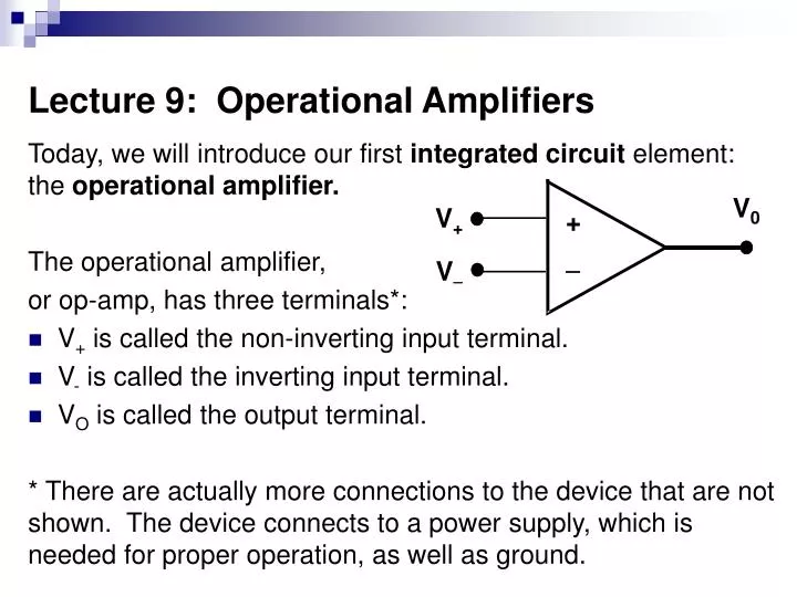
V0 V+ + V Lecture 9: Operational Amplifiers Today, we will introduce our first integrated circuit element: the operational amplifier. The operational amplifier, or op-amp, has three terminals*: • V+ is called the non-inverting input terminal. • V- is called the inverting input terminal. • VO is called the output terminal. * There are actually more connections to the device that are not shown. The device connects to a power supply, which is needed for proper operation, as well as ground.
+ + + V0 V1 Circuit Model in linear region Ro Ri AV1 I-V Relationship • The I-V relationship for the op-amp is complicated, since it has multiple terminals. • The op-amp can be modeled using the following circuit: • You can simply replace the op-amp symbol with the above circuit for analysis. • However, the above model is only valid when VO is within a certain range.
upper rail V0 lower rail Rails and Saturation • The output VO must lie within a range determined by the supply voltages, which are not shown. • It will limit or “clip” if VO attempts to exceed the boundaries. We call the limits of the output the “rails”. • In the linear region, the op-amp output voltage VO is equal to the gain A times the voltage across the input terminals. • You can “blindly” use the linear region model, and check if the output exceeds a rail. If so, the output is equal to that rail voltage. Slope is A
V0 VIN + + - V1 V0 + Ro + Ri AV1 VIN Example: Voltage Follower • Find the output voltage. Assume the rails are not exceeded.
+ + + V0 V1 Circuit Model Ro Ri AV1 Ideal Op-Amp Assumptions • While we can always use our circuit model for the linear region, it is complicated. • Ri is usually very large. • RO is usually very small. • A is usually very large (like 103 to 106). • Thus, we can make the following ideal assumptions for easier, but still pretty accurate, analysis: • Assume A = ∞. • Assume Ri = ∞. • Assume Ro = 0 W
V0 + V+ + V + + V1 V0 Ro Ri AV1 Ideal Op-Amp Model Our idealized op-amp follows these rules within the linear region: • Rule 1: V+ - V- = 0. • Why? If the output voltage is limited by rails, and the gain A is very large, then V+ - V- must be very small. • Rule 2: No current goes in/out of the input terminals. • Why? V+ - V- is very small and Ri is very large. • Remember current can go into/out the output terminal. • Why? There are connections not shown, and the current comes from those connections.
V0 VIN + Example: Voltage Follower • Find the output voltage. Assume the rails are not exceeded. VO = VIN
+ Utility of Voltage Follower • Suppose I have a voltage coming out of a digital circuit. • I want to apply the voltage to “turn on” some device that requires high power (the device “drains” a substantial amount of current). • Digital circuits usually cannot provide much current; they are designed for low power consumption. • If we put a voltage follower between the digital circuit and the load, the voltage follower replicates the desired voltage, and can also provide current through its power supply. Digital Circuit
Op-Amp Circuits • Op-Amp circuits usually take some input voltage and perform some “operation” on it, yielding an output voltage. • Some tips on how to find the output, given the input: Step 1: KVL around input loop (involves Vin and op-amp inputs) Use Rule 1: V+-V- = 0 Step 2: Find the current in the feedback path Use Rule 2: No current into/out of op-amp inputs Step 3: KVL around output loop (involves Vo and feedback path) Remember current can flow in/out op-amp output
VIN Example: Inverting Amplifier Feedback Path R2 R1 Input Loop V0 + Output Loop
R1 V1 RF R2 V2 V3 V0 R3 + Example: Inverting Summing Amplifier
R2 R1 Vo V IN Non-inverting Amplifier
Important Points • The amplifier output voltage does not depend on the “load” (what is attached to the output). • The “form” of the output voltage (the signs of the scaling factors on the input voltages, for example) depends on the amplifier circuit layout. • To change the values (magnitudes) of scaling factors, adjust resistor values. • Input voltages which are attached to the + (non-inverting) amplifier terminal get positive scaling factors. • Inputs attached to the – (inverting) terminal get negative scaling factors. • You can use these principles to design amplifiers which perform a particular function on the input voltages.
Example: Voltage Divider • Suppose I want to use the following circuit to supply a certain fraction of VIN to whatever I attach. • What is VO if nothing is attached? • What is VO if a 1 kW resistor is attached? • This circuit clearly does not supply the same voltage to any attached load. What could I add to the circuit so that it will supply the same fraction of VIN to any attached device?
Example • Design a circuit whose output is the sum of two input voltages.
Example • Design a circuit whose output is the average of two input voltages.