A multi plant problem

1. A multi plant problem A company consists of two factories A and B. Each factory makes two products: standard and deluxe Each unit of product yields the following profit Each factory use two processes, grinding and polishing for producing its product

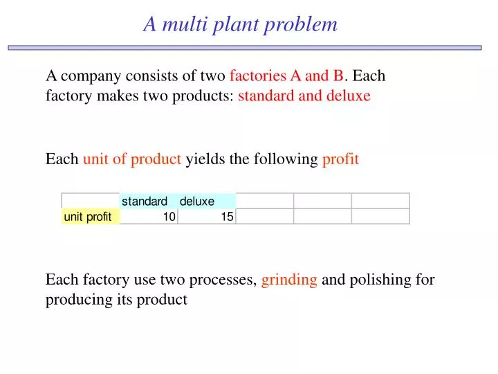
2. A multi plant problem The grinding and polishing times in hours for a unit of each type of product in each factory are Factory A has a grinding capacities of 80 hours per week and polishing capacity of 60 hours per week Factory B has a grinding capacities of 60 hours per week and polishing capacity of 75 hours per week

3. Factory A is allocated 75 Kg Factory B is allocated 45 Kg A multi plant problem Availability of raw material Each product (standard or deluxe) requires 4 kg of a raw material The company has 120 kg of raw material per week A possible scenario 120 kg.

4. Unit profit of standard product Unit profit of standard deluxe Kg of raw material for unit of standard product Kg of raw material for unit of deluxe product Mathematical model for factory A The two type of products are the decision variables for FACTORY A standard = x1, deluxe = x2 x1 , x2>= 0 Objective function is the profit to be maximize max 10x1 + 15 x2 Constraints: Availability of raw material 4x1 + 4 x2 <= 75

5. Mathematical model for factory A (2) Constraints: Technological constraints Grinding process 4x1 + 2 x2 <= 80 Polishing process 2x1 + 5 x2 <= 60 max 10x1 + 15 x2 4x1 + 4 x2 <= 75 4x1 + 2 x2 <= 80 2x1 + 5 x2 <= 60 x1 , x2 >= 0 Overall model for factory A

6. x2 All non negative points constitutes the 45 Feasible region 40 40 35 30 25 20 15 10 5 Bad use of resources ! x1 5 10 15 20 25 30 35 40 40 45 Geometric representation of F Let draw the set F of the feasible solutions for factory A In the plane (x1, x2 ), draw the equations of the constraints 4 x1 + 2 x2 = 80 The constraint 4 x1 + 2 x2 = 80 does not play any role in defining the feasible region: removing it does not change F 4 x1 + 4 x2 = 75 2 x1 + 5 x2 = 60

7. =0 x2 45 =150 40 40 35 =300 30 PTOT = 300 25 PTOT = 150 20 Find the value of PTOT such thatthe corresponding line “touch” the points 15 10 5 PTOT =0 5 10 15 20 25 30 35 40 40 45 Geometric representation of the profit In the plane (x1, x2 ), draw the equation of the profit PTOT for increasing values PTOT = 10x1 + 15 x2 They are parallel lines 4 x1 + 4 x2 = 75 PTOT =300 does not touch any point in F 2 x1 + 5 x2 = 60 x1

8. x2 45 40 Optimal solution 40 35 30 2 x1 + 5 x2 = 60 hours 25 4 x1 + 4 x2 = 75 Raw material 20 15 10 5 PTOT =0 5 10 15 20 25 30 35 40 40 45 Geometric solution In the plane (x1, x2 ), draw the parallel lines to the equationPTOT = 10x1 + 15 x2 =0 until the last point is found that “touches” the feasible region 4 x1 + 4 x2 = 75 PTOT = 10x1 + 15 x2 = 112.5 + 112.5 = 225 2 x1 + 5 x2 = 60 x1

9. Decision variables = level of production data x1=C9, x2 =D9 Profit = C4*C9+D4*D9 Raw constraint = C5*C9+D5*D9 Grinding constraint = C6*C9+D6*D9 Polishing constraint = C7*C9+D7*D9 Excel table for factory A

10. Objective function = profit Decision variables constraints Using the Solver

11. Mathematical model for factory B The two type of products are the decision variables for FACTORY B standard = x3, deluxe = x4 x3 , x4>= 0 Objective function is the profit to be maximize max 10x3 + 15 x4 Constraints: Availability of raw material 4x3 + 4 x4 <= 45

12. Grinding process 5x3 + 3 x4 <= 60 Polishing process 5x3 + 6 x4 <= 75 Mathematical model for factory B (2) Constraints: Technological constraints max 10x3 + 15 x3 4x3 + 4 x3 <= 45 5x3 + 3 x4 <= 60 5x3 + 6 x4 <= 75 x3, x3 >= 0 Overall model for factory B

13. x4 All non negative points constitutes the 50 Feasible region 40 30 20 15 10 5 Bad use of resources ! x3 5 10 15 20 30 40 50 Geometric representation of F Let draw the set F of the feasible solutions for factory B In the plane (x3, x4 ), draw the equations of the constraints Two constraints 5 x3 + 6 x4 = 75and 5 x3 + 3 x4 = 60 do not play any role in defining the feasible region: removing them does not change F 5 x3 + 3 x4 = 60 4 x3 + 4 x4 = 45 5 x3 + 6 x4 = 75

14. x4 50 40 30 Find the value of PTOT such thatthe corresponding line “touch” the points x3 = 0 20 Optimal solution = 15 Raw material 4 x3 + 4 x4 = 45 10 5 PTOT =0 x3 5 10 20 30 40 50 Geometric solution In the plane (x3, x4 ), draw the parallel equations of the profit PTOT for increasing values =0 PTOT = 10x3 + 15 x4 =100 4 x3 + 4 x4 = 45 PTOT = 112.5 PTOT = 100

15. Decision variables = level of production data x3=C9, x4 =D9 Profit = C4*C9+D4*D9 Raw constraint = C5*C9+D5*D9 Grinding constraint = C6*C9+D6*D9 Polishing constraint = C7*C9+D7*D9 Excel table for factory B Note: the excel formulae are the same for factory A and B. The model is independent from data

16. Overall production = sum of the production of factory A and factory B Profit of the company = sum of the profits of factory A and factory B Look at the company in this scenario This solution has been obtained witharbitrary allocation of resources

17. Total raw material Factory A is allocated 90 Kg 120 kg. Factory B is allocated 30 Kg Changing the scenario The solution has been obtained witharbitrary allocation of raw material, we can see what happens when allocation change

18. x2 5 x3 + 3 x4 = 60 x4 50 50 4 x1 + 2 x2 = 80 45 40 40 4 x3 + 4 x4 = 30 4 x1 + 4 x2 = 90 30 30 5 x3 + 6 x4 = 75 20 x2 20 x4 2 x1 + 5 x2 = 60 x1 15 15 new optimum for A 20 20 10 15 15 10 10 5 5 5 5 x1 x3 x3 50 5 5 10 10 15 15 20 20 30 30 40 40 50 5 10 15 20 5 10 15 20 Changing the scenario: geometric view Factory A Factory B new optimum for B PTOT = 250 PTOT = 112.5

19. Factory A Profit is higher than the preceding scenario Factory B Profit is lower than the preceding scenario Changing the scenario: excel view

20. Overall production = sum of the production of factory A and factory B Profit of the company = sum of the profits of factory A and factory B Look at the company in the new scenario This solution is worst than the preceding one

21. standard in factory A= x1, deluxe in factory A = x2standard in factory B= x3, deluxe in factory B= x4 x1 , x2,x3 , x4>= 0 Objective function is the overall profit to be maximize max 10x1 + 15 x2 +10x3 + 15 x4 Mathematical model for the company The two type of products produced in FACTORY A and B are the decision variables

22. Factory A Factory B Factory A Factory B 4x1 + 4 x2 +4x3 + 4 x4 <= 120 Common constraint Mathematical model for the company (2) Constraints: Technological constraints Grinding process 4x1 + 2 x2 <= 80 5x3 + 3 x4 <= 60 Polishing process 2x1 + 5 x2 <= 60 5x3 + 6 x4 <= 75 Constraints: Availability of raw material

23. Mathematical model for the company max10x1 + 15 x2 +10x3 + 15 x4 4x1 + 2 x2 <= 80 5x3 + 3 x4 <= 60 2 x1 + 5 x2 <= 60 5 x3 + 6 x4 <= 75 4 x1 + 4 x2 + 4x3 + 4 x4 <= 120 x1 , x2,x3 , x4>= 0 More than two variables: we can solve it with the Solver

24. Decision variables = level of production x1=C10, x2 =D10, x3=E10, x4 =F10 Profit = C4*(C10+E10)+D4*(D10+F10) Raw constraint = C5*(C10+ E10 )+D5*(D10+F10) Excel table for the company

25. Setting the solver

26. Optimal production: deluxe = 20.8, standard = 9.17 Profit = 404.16 Optimal solution for the company Better than 393.75 obtained with the arbitrary allocation