Download
1 / 80
800 likes | 806 Views
Comparing k Populations. Means – One way Analysis of Variance (ANOVA). The F test – for comparing k means. Situation We have k normal populations Let m i and s denote the mean and standard deviation of population i . i = 1, 2, 3, … k .

E N D
Comparing k Populations Means – One way Analysis of Variance (ANOVA)
The F test – for comparing k means Situation • We have k normal populations • Let miand s denote the mean and standard deviation of population i. • i = 1, 2, 3, … k. • Note: we assume that the standard deviation for each population is the same. s1 = s2 = … = sk = s
We want to test against
The data • Assume we have collected data from each of th k populations • Let xi1, xi2 , xi3 , … denote the ni observations from population i. • i = 1, 2, 3, … k. Let
One possible solution (incorrect) • Choose the populations two at a time • then perform a two sample t test of • Repeat this for every possible pair of populations
The flaw with this procedure is that you are performing a collection of tests rather than a single test • If each test is performed with a= 0.05, then the probability that each test makes a type I error is 5% but the probability the group of tests makes a type I error could be considerably higher than 5%. • i.e. Suppose there is no different in the means of the populations. The chance that this procedure could declare a significant difference could be considerably higher than 5%
The Bonferoni inequality If N tests are preformed with significance level a. then P[group of N tests makes a type I error] ≤ 1 – (1 – a)N Example: Suppose a. = 0.05, N = 10 then P[group of N tests makes a type I error] ≤ 1 – (0.95)10= 0.41
For this reason we are going to consider a single test for testing: against Note: If k = 10, the number of pairs of means (and hence the number of tests that would have to be performed ) is:
To test against use the test statistic
the statistic is called the Between Sum of Squares and is denoted by SSBetween It measures the variability between samples k – 1 is known as the Between degrees of freedom and is called the Between Mean Square and is denoted by MSBetween
the statistic is called the Within Sum of Squares and is denoted by SSWithin is known as the Within degrees of freedom and is called the Within Mean Square and is denoted by MSWithin
The Computing formula for F: Compute 1) 2) 3) 4) 5)
Then 1) 2) 3)
The critical region for the F test We reject if Fais the critical point under theF distribution with n1 = k - 1degrees of freedom in the numerator and n2 = N – k degrees of freedom in the denominator
Example In the following example we are comparing weight gains resulting from the following six diets • Diet 1 - High Protein , Beef • Diet 2 - High Protein , Cereal • Diet 3 - High Protein , Pork • Diet 4 - Low protein , Beef • Diet 5 - Low protein , Cereal • Diet 6 - Low protein , Pork
Thus Thus since F > 2.386 we reject H0
The ANOVA Table A convenient method for displaying the calculations for the F-test
Equivalence of the F-test and the t-test when k = 2 the t-test
Using SPSS Note: The use of another statistical package such as Minitab is similar to using SPSS
Each variable is in a column • Weight gain (wtgn) • diet • Source of protein (Source) • Level of Protein (Level)
After starting the SSPS program the following dialogue box appears:
If you select Opening an existing file and press OK the following dialogue box appears
If the variable names are in the file ask it to read the names. If you do not specify the Range the program will identify the Range: Once you “click OK”, two windows will appear
To perform ANOVA select Analyze->General Linear Model-> Univariate
Select the dependent variable and the fixed factors Press OK to perform the Analysis
Comments • The F-test H0: m1 = m2 = m3 = … = mk against HA: at least one pair of means are different • If H0 is accepted we know that all means are equal (not significantly different) • If H0 is rejected we conclude that at least one pair of means is significantly different. • The F – test gives no information to which pairs of means are different. • One now can use two sample t tests to determine which pairs means are significantly different
Fishers LSD (least significant difference) procedure: • Test H0: m1 = m2 = m3 = … = mk against HA: at least one pair of means are different, using the ANOVA F-test • If H0 is accepted we know that all means are equal (not significantly different). Then stop in this case • If H0 is rejected we conclude that at least one pair of means is significantly different, then follow this by • using two sample t tests to determine which pairs means are significantly different
Example In the following example we are comparing weight gains resulting from the following six diets • Diet 1 - High Protein , Beef • Diet 2 - High Protein , Cereal • Diet 3 - High Protein , Pork • Diet 4 - Low protein , Beef • Diet 5 - Low protein , Cereal • Diet 6 - Low protein , Pork
The ANOVA Table Thus since F > 2.386 we reject H0 Conclusion: There are significant differences amongst the k = 6 means
Now we want to perform t tests to compare the k = 6 means with t0.025= 2.005 for 54 d.f.
Table of means t test results Critical value t0.025= 2.005 for 54 d.f. t values that are significant are indicated in bold.
Conclusions: • There is no significant difference between diet 1 (high protein, pork)and diet 3 (high protein, pork). • There are no significant differences amongst diets 2, 4, 5 and 6. (i. e. high protein, cereal (diet 2) and the low protein diets (diets 4, 5 and 6)). • There are significant differences between diets 1and 3 (high protein, meat) and the other diets (2, 4, 5, and 6). • Major conclusion: High protein diets result in a higher weight gain but only if the source of protein is a meat source.