Download
1 / 24
310 likes | 616 Views
Scale Invariant Feature Transform (SIFT). Outline. What is SIFT Algorithm overview Object Detection Summary. Overview. 1999 Generates image features, “keypoints” invariant to image scaling and rotation partially invariant to change in illumination and 3D camera viewpoint

E N D
Outline • What is SIFT • Algorithm overview • Object Detection • Summary
Overview • 1999 • Generates image features, “keypoints” • invariant to image scaling and rotation • partially invariant to change in illumination and 3D camera viewpoint • many can be extracted from typical images • highly distinctive
Algorithm overview • Scale-space extrema detection • Uses difference-of-Gaussian function • Keypoint localization • Sub-pixel location and scale fit to a model • Orientation assignment • 1 or more for each keypoint • Keypoint descriptor • Created from local image gradients
Scale space • Definition: where
Scale space • Keypoints are detected using scale-space extrema in difference-of-Gaussian function D • D definition: • Efficient to compute
Relationship of D to • Close approximation to scale-normalized Laplacian of Gaussian, • Diffusion equation: • Approximate ∂G/∂σ: • giving, • When D has scales differing by a constant factor it already incorporates the σ2 scale normalization required for scale-invariance
Scale space construction 2k2σ 2kσ 2σ kσ σ 2kσ 2σ kσ σ
Scale space images … … … … … first octave … second octave … third octave … fourth octave
Difference-of-Gaussian images … … … … … first octave … second octave … third octave … fourth octave
Frequency of sampling • There is no minimum • Best frequency determined experimentally
Prior smoothing for each octave • Increasing σ increases robustness, but costs • σ = 1.6 a good tradeoff • Doubling the image initially increases number of keypoints
Finding extrema • Sample point is selected only if it is a minimum or a maximum of these points Extrema in this image DoG scale space
Localization • 3D quadratic function is fit to the local sample points • Start with Taylor expansion with sample point as the origin • where • Take the derivative with respect to X, and set it to 0, giving • is the location of the keypoint • This is a 3x3 linear system
Localization • Derivatives approximated by finite differences, • example: • If X is > 0.5 in any dimension, process repeated
Filtering • Contrast (use prev. equation): • If | D(X) | < 0.03, throw it out • Edge-iness: • Use ratio of principal curvatures to throw out poorly defined peaks • Curvatures come from Hessian: • Ratio of Trace(H)2 and Determinant(H) • If ratio > (r+1)2/(r), throw it out (SIFT uses r=10)
Orientation assignment • Descriptor computed relative to keypoint’s orientation achieves rotation invariance • Precomputed along with mag. for all levels (useful in descriptor computation) • Multiple orientations assigned to keypoints from an orientation histogram • Significantly improve stability of matching
Descriptor • Descriptor has 3 dimensions (x,y,θ) • Orientation histogram of gradient magnitudes • Position and orientation of each gradient sample rotated relative to keypoint orientation
Descriptor • Weight magnitude of each sample point by Gaussian weighting function • Distribute each sample to adjacent bins by trilinear interpolation (avoids boundary effects)
Descriptor • Best results achieved with 4x4x8 = 128 descriptor size • Normalize to unit length • Reduces effect of illumination change • Cap each element to 0.2, normalize again • Reduces non-linear illumination changes • 0.2 determined experimentally
Object Detection • Create a database of keypoints from training images • Match keypoints to a database • Nearest neighbor search
PCA-SIFT • Different descriptor (same keypoints) • Apply PCA to the gradient patch • Descriptor size is 20 (instead of 128) • More robust, faster
Summary • Scale space • Difference-of-Gaussian • Localization • Filtering • Orientation assignment • Descriptor, 128 elements