Download

1 / 86
880 likes | 1.01k Views
Introduction to Production and Resource Use. Chapter 6. Topics of Discussion. Conditions of perfect competition Classification of inputs Important production relationships (assume one variable input in this chapter) Assessing short-run business costs Economics of short-run decisions.

E N D
Topics of Discussion • Conditions of perfect competition • Classification of inputs • Important production relationships (assume one variable input in this chapter) • Assessing short-run business costs • Economics of short-run decisions
Conditions for Perfect Competition • Homogeneous products • No barriers to entry or exit • Large number of sellers • Perfect information Page 86
Classification of Inputs • Land:includes renewable (forests) and non-renewable (minerals) resources • Labor:all owner and hired labor services, excluding management • Capital:manufactured goods such as fuel, chemicals, tractors and buildings • Management:production decisions designed to achieve specific economic goal Pages 86-87
Production Function Output = f(labor|capital, land, and management) Start with one variable input Page 88
Production Function Output = f(labor|capital, land, and management) Start with one variable input assume all other inputs fixed at their current levels… Page 112
Coordinates of input and output on the TPP curve Page 89
Total Physical Product (TPP) Curve Variable input Page 89
Law of DiminishingMarginal Returns “As successive units of a variable input are added to a production process with the other inputs held constant, the marginal physical product (MPP) eventually declines” Page 93
Other Physical Relationships The following derivations of the TPP curve play An important role in decision-making: Marginal Physical = Output ÷ Input Product Pages 90
Other Physical Relationships The following derivations of the TPP curve play An important role in decision-making: Marginal Physical = Output ÷ Input Product Average Physical = Output ÷ Input Product Pages 90-91
Change in output as you increase inputs Page 89
Total Physical Product (TPP) Curve Marginal physical product is .45 as labor is increased from 16 to 20 output input Page 89
Output per unit input use Page 89
Total Physical Product (TPP) Curve Average physical product is .31 if labor use is 26 output input Page 89
Plotting the MPP curve Change in output associated with a change in inputs Page 91
Marginal Physical Product Change from point A to point B on the production function is an MPP of 0.33 Page 91
Plotting the APP Curve Level of output divided by the level of input use Page 91
Average Physical Product Output divided by labor use is equal to 0.19 Page 91
Three Stages of Production Average physical product (yield) is increasing in Stage I Page 91
Three Stages of Production Marginal physical product falls below the average physical product in Stage II Page 91
Three Stages of Production MPP goes negative in stage III… Page 91
Three Stages of Production Why are Stage I and Stage III irrational? Page 91
Three Stages of Production Output falling Productivity rising so why stop??? Page 91
Three Stages of Production The question therefore is where should I operate in Stage II? Page 114
Economic Dimensions • We need to account for the price of the product • We also need to account for the cost of the inputs
Key Cost Relationships The following cost derivations play a key role in decision-making: Marginal cost = total cost ÷ output Page 117-120
Key Cost Relationships The following cost derivations play a key role in decision-making: Marginal cost = total cost ÷ output Average variable = total variable cost ÷ output cost Page 117-120
Key Cost Relationships The following cost derivations play a key role in decision-making: Marginal cost = total cost ÷ output Average variable = total variable cost ÷ output cost Average fixed = total fixed cost ÷ output cost Average total = total cost ÷ output = AVC+AFC cost Pages 94-96
From TPP curve on page 113 Page 94
Fixed costs are $100 no matter the level of production Page 94
Column (2) divided by column (1) Page 94
Costs that vary with level of production Page 94
Column (4) divided by column (1) Page 94
Column (2) plus column (4) Page 94
Change in column (6) associated with a change in column (1) Page 94
Column (6) divided by column (1) or Page 94
or column (3) plus column (5) Page 94
Plotted cost relationships from table 6.3 on page 94 Plotting costs for levels of output Page 95
Now let’s assume this firm can sell its product for $45/unit
Key Revenue Concepts Notice the price in column (2) is identical to marginal revenue in column (7). What about average revenue, or AR? What do you see if you divide total revenue in column (3) by output in column (1)? Yes, $45. Thus, P = MR = AR under perfect competition. Page 98
$45 P=MR=AR Profit maximizing level of output, where MR=MC 11.2 Page 99
Average Profit = $17, or AR – ATC P=MR=AR $45-$28 $28 Page 99
Grey area represents total economic profit if the price is $45… P=MR=AR 11.2 ($45 - $28) = $190.40 Page 99
P=MR=AR Zero economic profit if price falls to PBE. Firm would only produce output OBE . AR-ATC=0 Page 99
P=MR=AR Economic losses if price falls to PSD. Firm would shut down below output OSD Page 99
Where is the firm’s supply curve? P=MR=AR Page 99
Marginal cost curve above AVC curve? P=MR=AR Page 99