Download
1 / 53
670 likes | 1k Views
Heat Exchanger Network Retrofit. Trevor Hallberg Sarah Scribner. Heat Exchanger Network (HEN) Retrofit. Outline Mixed Integer Linear Programming (MILP) Pinch Technology Theory for Retrofit Improvements on Pinch Technology Crude Distillation Unit Example Discussion. CU. 128 ˚C. 35.5 ˚C.

E N D
Heat Exchanger NetworkRetrofit Trevor Hallberg Sarah Scribner
Heat Exchanger Network (HEN)Retrofit • Outline • Mixed Integer Linear Programming (MILP) • Pinch Technology Theory for Retrofit • Improvements on Pinch Technology • Crude Distillation Unit Example • Discussion
CU 128˚C 35.5˚C 10 kW/°C H1 1 2 5 30˚C 170°C 55 kW HU 76.7˚C 9 kW/°C 30˚C C1 1 200°C 3 1110 kW 420 kW HU 109.1˚C 11 kW/°C C2 200˚C 4 2 25˚C 925 kW 1000 kW Heat Exchanger Network (HEN)Retrofit • Retrofit Options : • Adjust existing area • Relocate existing exchangers • Add new exchangers • Introduce stream splits • Optimal Results : • Reduce utility usage • Increase process-process exchange • Maintain network integrity • Small Conceptual Example
Mixed Integer Linear Programming (MILP) Hot stream, i Cold stream, j 3 4 5 6 7 8 • Heat transfer Zones • Temperature Intervals • Energy and flow balances Based on transportation-transshipment model
Mixed Integer Linear Programming(MILP) • Heat Transfer Zones • Two Zones • Pinch Technology (Above and Below the Pinch) • One Zone • Find minimum total cost, even if cross-pinch transfer occurs
MILP • Sophisticated cost analysis • Model parameters • Area adjustment • Existing heat exchangers • New heat exchangers • Re-piping • Ability to tailor-fit model for a variety of HEN scenarios
Area Adjustments • Area Reduction • Plug Tubes • By-pass fluid • Enforce realistic area adjustments • Area reduction ≤ 50% • Area Addition • Existing Exchangers • Increase area of existing shell • Install a new, larger shell • New Exchangers • Limit number of new exchangers • Limit area (size) of new exchangers • Enforce realistic area adjustments • Area addition ≤ 20%
Re-piping • Re-piping scenarios • Exchanger relocation • Stream splitting • Exchanger by-pass • Re-piping cost assignments • Model compares number of split streams in retrofitted network to original network • Assigns user-defined fixed cost to number of new splits
MILP • Objective Functions • Maximize value of savings • Value of Savings = Utility Cost Savings – Annual Capital Cost • Maximize net present value • NPV = ∑(DiscountFactori * Utility Cost Savingsi ) – Capital Cost • Maximize return on investment • ROI = Annual Utility Cost Savings / Capital Cost
MILP • INPUT Parameters • Stream data (F·Cp) • Stream temperatures (Inlet & Target) • Cost functions • OUTPUT Data • Optimized objective function • Exchanger locations • Cost requirements • Utility savings
Pinch Technology • The root of heat integration technology • Systematic methodology for retrofitting • Identifies locations where process change will reduce the overall energy consumption • Allows us to set these energy targets • Allows us to set total cost targets
Pinch Technology • Based on thermodynamic principles • Uses Temperature vs. Enthalpy diagrams • Called composite curves
Pinch Technology Composite Curves - Combined
Pinch Technology • The pinch (ΔTmin) • Splits the process into 2 regions that are analyzed separately • “Heat Sink” region above the pinch • “Heat Source” region below the pinch
Pinch Technology • Violating these results in cross-pinch heat transfer • Increases heat requirements • 3 Pinch Rules • No heat transfer across the pinch • No external cooling above the pinch (only HU) • No external heating below the pinch (only CU)
Pinch Technology • Total Network Area - Aideal • Q = U•Ainterval•ΔTLM • “Vertical Heat Transfer”- vertical enthalpy regions • Assumes equal area of each exchanger • Vary ΔTmin • Aideal = A1+A2+…+Ai
Pinch Technology • Retrofitting • Energy vs. Area diagram • Blue curve = Aideal for various ΔTminvalues • Want to improve ineffective use of area • Want to decrease energy requirements
Pinch Technology • Retrofitting continued • Why would we increase area and energy? • Could theoretically work but the point is to use area better and decrease energy • Pinch recommends not decreasing area in which we have already invested - ??? • For now we will assume this is our retrofit path
Pinch Technology • Need a way to compare energy and area Which path do we choose? • Want a curve similar to the optimum design curve • Need a way to determine the most economical solution on the new curve • We use something called area efficiency
Pinch Technology • Area Efficiency (α) • Based on utilities of current process • Agrassroots = optimal area for current process • Assume new design has αnew ≥ αcurrent • The best α can be is 1 (cannot be better than ideal)
Pinch Technology Aretrofit Aexisting Aideal Agrassroots • Can now calculate Aretrofitbased on constant curve • Process: ΔTmin Qu,min Aideal Aretrofit • Area Efficiency • Assume α = βand
Pinch Technology • Which α do we use? • Infinite amount of α values • At least want αcurrent • The best is α = 1 • Larger α = smaller Aretrfit • Assume value of 1
Pinch Technology • Now that we have Aretrofit? • We need the optimum ΔTmin value • Total Annualized Cost (TAC) vs. ΔTmin diagram for constant α • Optimum ΔTmin value corresponds to the minimum
Pinch Technology • TAC vs. ΔTmin • Nmin = [Nh+Nc+Nu-1]AP + [Nh+Nc+Nu-1]BP • Still assuming that the total area of the network is distributed evenly among the exchangers
35.5˚C CU 128˚C 40˚C 40˚C 10 kW/°C H1 1 2 5 30˚C 170°C 55 kW HU 76.7˚C 30˚C 30˚C 11 kW/°C C1 1 200°C 3 1110 kW 420 kW HU 30˚C 30˚C 109.1˚C 9kW/°C C2 200˚C 4 2 25˚C 925 kW 1000 kW Pinch Technology • Now we need to design the HEN • Eliminate cross-pinch heat exchangers (E2) • Reuse the other exchangers (usually more economic) • Design sections above and below pinch separately
35.5˚C CU 128˚C 40˚C 40˚C 10 kW/°C H1 1 2 5 30˚C 170°C 45 kW HU 76.7˚C 30˚C 30˚C 11 kW/°C C1 1 200°C 3 230 kW 1300 kW HU 30˚C 30˚C 109.1˚C 9 kW/°C C2 200˚C 4 25˚C 2 55 kW 1870 kW Pinch Technology • Maximize exchanger loads • Q = F•Cp•ΔT (for each stream) • HEN Design • Start design at pinch • Matching streams • AP: (F•Cp)hot ≤ (F•Cp)cold • BP: (F•Cp)cold ≤ (F•Cp)hot
35.5˚C CU 128˚C 40˚C 40˚C 10 kW/°C H1 6 1 2 5 30˚C 170°C 45 kW HU 76.7˚C 30˚C 30˚C 11 kW/°C C1 1 200°C 3 1300 - X kW 230 + X kW HU 30˚C 30˚C 109.1˚C 9kW/°C C2 200˚C 4 25˚C 6 2 55 kW 1870 - X kW Pinch Technology X kW • HEN Design • Add E6 to reduce utilities • Use loops and paths to make design more flexible • Give E6 a duty of X • A web of exchangers is affected
Pinch Technology • Individual Heat Exchanger Area • Evaluate the specific exchanger areas by accounting for temperature cross within the exchangers • Need these areas to calculate the capital cost
Pinch Technology • Cost comparisons • No longer assume equal areas for each exchanger • CC (Capital Investment Cost) • Based on area change for each exchanger in the network • Fixed and variable costs • Includes area addition, reduction, and new exchanger cost • Operating Costs (OC) • ∆TAC (Total Annualized Cost) • ROI (Return on Investment)
Pinch Technology • How can we improve it? • Allowing relocation of all exchangers • May be able to cut down on area change expenses • May decrease the number of new exchangers needed • Incorporate Pro-II simulation
Pinch Technology Improvement • Incorporate Pro-II Optimization • Pro-II simulation based on Pinch Technology results • Exchanger location • Minimize total cost • Vary heat exchanger area • Vary stream split ratio • Fix stream target temperatures
Pro-II Optimization • Controllers set stream target temps Calculator assigns cost equations Optimizer minimizes cost function
HEN Retrofit Results • Crude Distillation Unit • MILP • Process Pinch • Process Pinch Improvements • Pro-II Simulation • Retrofit Considerations • Stream splitting • Addition of new exchangers • Allow & disallow exchanger relocation
Crude Distillation Unit • Original Network • 10 Hot streams • 3 Cold streams • 18 exchangers • 2 hot utilities • 3 cold utilities
Original MILP Process Pinch • COMPARISON • Original • 18 exchangers • MILP • 8 new exchangers • Process Pinch • 9 new exchangers No Relocation Allowed
Original MILP Process Pinch • COMPARISON • Original • 18 exchangers • MILP • 5 new exchangers • 5 relocated • Process Pinch • 9 new exchangers • 7 relocated Allow Relocation
Discussion • Computation Time Comparison • MILP is most time-efficient • MILP only requires input of data • Pro-II requires large majority of manual labor • Pinch requires manual labor only
Where Does Pinch Go Bad? We believe the problem is with ΔTmin The optimum value is determined prior to design Assumes equal area of every exchanger Optimization occurs after the value is chosen
MILP = The Best • Why? • Considers the greatest number of variables • Considers all solutions • No limiting assumptions or methodology • Optimization based on several cost parameters • Computer does everything a person can do • Only requires input of data • Do not need experience with the methodology
Process Pinch Limitations • Why does pinch overlook MILP solutions? • Optimum solution based on min number of units • It then optimizes the area distribution and utilities • For large networks, there are many (if not infinite) combinations of exchangers and heat loads to satisfy a process • Cannot efficiently consider all heat loops and paths
228.5 H1 3 5 77˚ 159 0 CU 20.4 H2 267˚ 4 6 88˚ CU 53.8 343˚ H3 1 2 90˚ 93.3 26˚ 127 0 C1 HU 196.1 118˚ 265˚ 7 C2 Example 1 • Original Network • 7 exchangers • 1 heater (E7) • 2 coolers (E5,E6)
New +A -A H1 159 0 8 3 77˚ +A New 267˚ 4 H2 88˚ 9 -A +A 343˚ 2 H3 1 90˚ NEW SPL 127 0 26˚ C1 +A NEW SPL 118˚ 265˚ C2 Example 1- Process Pinch 5 CU 6 CU HU 7 • Retrofitted Network (No relocation Allowed) • 8 exchangers (E6 becomes non-operational) • 1 heater (E7), 1 cooler (E5) • E8 and E9 added to increase process exchange
Example 1 – Process Pinch New +A -A H1 159 0 8 3 77˚ +A 267˚ 4 H2 88˚ 6 -A +A 343˚ 2 H3 1 90˚ NEW SPL 127 0 26˚ C1 +A NEW SPL 118˚ 265˚ C2 5 +A CU 6 CU HU 7 • Retrofitted Network (Relocation Allowed) • 8 exchangers (E6 is relocated a process exchanger) • 1 heater (E7), 1 cooler (E5) • E8 added to meet increase process exchange
H1 159˚ 8 3 5 77˚ -A New CU 267˚ H2 4 9 6 88˚ CU New +A , NS -A H3 1 2 90˚ 343˚ +A , NS +A, NS NEW SPL 26˚ 127˚ C1 NEW SPL HU -A C2 7 118˚ 265˚ Example 1- MILP • Retrofitted Network (No relocation Allowed) • 9 exchangers • 1 heater (E7), 2 coolers (E5, E6) • E8,E9 added to increase process exchange
CU I1 5 8 159˚ 5 77˚ 3 +A New CU 267˚ I2 6 4 6 9 88˚ +A, NS New CU I3 1 2 10 90˚ 343˚ New +A, NS 127˚ 26˚ J1 NEW SPL HU 7 J2 118˚ 265˚ -A Example 1- MILP • Retrofitted Network (Relocation Allowed) • 9 exchangers • 1 heater (E7), 2 coolers (E5, E6) • E8,E9 added to increase process exchange
Example 1 • Results (No relocation) • MILP has 1 more exchanger than pinch • MILP has more area but requires less energy • Pinch has less area but requires more energy • Pro-II simulation further optimizes the pinch technology