Download
1 / 14
170 likes | 385 Views
Primitives pt/line/conic HZ 2.2. Behaviour at infinity. Projective transform HZ 2.3. Hierarchy of maps Invariants HZ 2.4. DLT alg HZ 4.1. Rectification HZ 2.7. Projective transform 1. now that we have this new projective space, let’s understand how to transform it

E N D
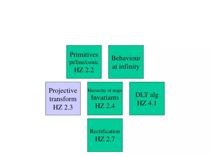
Primitives pt/line/conic HZ 2.2 Behaviour at infinity Projective transform HZ 2.3 Hierarchy of maps Invariants HZ 2.4 DLT alg HZ 4.1 Rectification HZ 2.7
Projective transform 1 • now that we have this new projective space, let’s understand how to transform it • necessary to understand how a camera transforms space • a projective transform is a linear map in projective space • projective transform = projectivity = homography = collineation • it can encode perspective projection and the image formation process of the pinhole camera • Euclidean transform cannot • Euclidean transform = translation + rotation = rigid transform • we will study projective transform and some special cases • some properties are preserved (invariant) and others are not • collinearity is, angle is not (and so parallel lines are not) • we will study invariants of the various types of map
What is a projective transform? • Preferred definition (matrix-based): A projective transform is a map h:P^2 P^2, h(x) = Hx where H is a nonsingular 3x3 matrix. • Alternate definition (line preservation): A projective transform is an invertible map h:P^2 P^2 that preserves lines. • i.e., x1,x2,x3 lie on same line iff h(x1), h(x2), h(x3) do • invertibility means that map is one-to-one and onto • first definition is algebraic, second is geometric • proof of equivalence (actually just the reduction from algebraic to geometric) • let h(x)=Hx be a projective transform, then • x_i lie on the line L Lx_i = 0 L H^{-1}Hx_i Hx_i lie on the line LH^{-1} • so h(x) preserves lines • recall that L is a row vector • Corollary: when points transform as x Hx, lines transform as L LH^{-1} • important; foreshadowing of tensor (contravariant vs. covariant transformation)\ • this result is used to map the vanishing line to the line at infinity and then map pixels accordingly (since pixels are points, not lines) • HZ32-34
Projective transform 2 • in 1st definition, H is a homogeneous matrix, since scaling does not change the map • H has 8 dof • question: how many dof do a point, line and conic have? • the geometric definition motivates the term ‘collineation’ • homographies form a group • can be composed, have an identity, have an inverse • generalization: a map from P^3 to P^3, or from P^3 to P^2, that preserves lines is also called a homography • note that the equivalence to nonsingular matrix algebraic definition does not hold for maps from P^3 to P^2 (e.g., perspective projection matrix is singular) • exercise: why is perspective projection a homography?
Perspective projection • perspective projection is a homography • preserves lines: given a line L in 3-space, consider the plane through L and C (camera center); a plane intersects a plane in a line • yet persp(X,Y,Z,1) = (diag(f,f,1) 0) (X,Y,Z,1) so matrix definition does not apply • indeed, a special case of a homography • interesting fact: composition of two perspectivities is not a perspectivity • perspectivity = perspective projection between two planes
Day x: (A growing list of) key facts in projective geometry • L1 x L2: line intersection • P1 x P2: point join • P.L = 0: point/line incidence • line at infinity (0,0,1) • finding vanishing line with 7 cross products • homography encoded by 3x3 matrix H • if P HP, then L LH^{-1} • circular points I, J = (1, \pm i, 0)
Structure from motion diagram Projective geometry Camera geometry Two-view geometry Three-view geometry n-view geometry Calibration
Primitives pt/line/conic HZ 2.2 Behaviour at infinity Projective transform HZ 2.3 Hierarchy of maps Invariants HZ 2.4 DLT alg HZ 4.1 Rectification HZ 2.7
Classes of homography • from most restrictive to most general • Euclidean transform = rigid transform • translation and rotation only • move the origin and rotate the coordinate frame • similarity transform: also isometrically scale • affine transform: allow different scaling in coordinate directions • linear transform of Euclidean space (i.e., not ideal points), then Euclidean transform • none of these transforms affect line at infinity: ideal points remain at infinity • in contrast, all points are created equal with projective transform: ideal points may map to finite points • projective transform = linear transform of projective space • HZ 2-3
Similarity and metric structure • we are most interested in similarity transforms, since we shall define the structure of a scene up to a similarity • metric structure = structure defined up to a similarity • it is impossible to know the absolute position or orientation of an imaged object, or its scale • is this picture of Sam sitting at a desk taken in New York or Casablanca, on the third floor or tenth, leaning backward or sitting up straight? is this imaged Millenium Falcon in outer space 26.7 meters long or 19.33 inches long? • context might give an indication of scale (e.g., height of door, orientation of door, known landmark in picture) • therefore, the best we can expect, and our goal, is to retrieve the metric structure of the object • if G is the true geometry of the object and G’ is our reconstructed geometry, then G = SG’ for some similarity S
Invariants • Euclidean: length and area • similarity: angle, ratio of length and area • affine: parallelism • e.g., reflection of stained glass on wall • projective: collinearity, order of contact (e.g., intersection, tangency) • initially, we shall restore structure only up to a projective transform (not a similarity) • for example, a cube may be reconstructed simply as a polyhedron (not even a parallelepiped) • metric reconstruction = reconstruction up to a similarity • projective reconstruction = reconstruction up to a homography • for metric reconstruction, we shall need to calibrate • rectification is a 2d analog of metric reconstruction
As matrices • projective transforms PL(3): homogeneous nonsingular 3x3 matrices • Euclidean: [R t; 0,0,1]; upper left 2x2 submatrix is orthogonal • motivation: don’t want to stretch space, leave 3rd coordinate alone • translation vector is 3rd column; rotation or rotation/reflection is 2x2 • orientation-preserving Euclidean if det=1 (models rigid motion) • assume orientation-preserving: realistic transforms are • similarity: [sR t; 0 1] • affine: [A; 0, 0 1]; 3rd row is identity (0,0,1) • A = [K t], no restriction on K • motivation: want ideal points to remain ideal • Euclidean transform has 3dof (1 rotation, 2 translation) • similarity has 4dof • HZ37-39
A similarity fixes the circular points • What characterizes a similarity? • Theorem: A projective transform is a similarity iff the circular points are fixed. • Proof: • Let H = [s cos,-s sin,tx; s sin, s cos, ty; 0 0 1] be a similarity. H(1,i,0) = s (cos- i sin, sin+i cos,0). Recall that c(theta)+is(theta) = e^{i theta}. So H(1,i,0) = s(e^{i –theta}, i e^{i –theta},0) = se^{-i theta} (1,i,0) = (1,i,0) • Homework 1 • Resulting strategy: we can change a projective transform into a similarity by finding the imaged circular points and moving them back to the true circular points (ensuring that the circular points are fixed) • intuition: not surprising that metric properties like angle can be restored once circular points are known: • I = (1,0,0) + i (0,1,0) = concise package of the two coordinate directions
Goal: finding circular points • this motivates finding the images of the circular points I,J for metric rectification • it is easier to find a certain dual conic (a line conic dual to the circular points) • this requires an exploration of conics