Download
1 / 23
230 likes | 322 Views
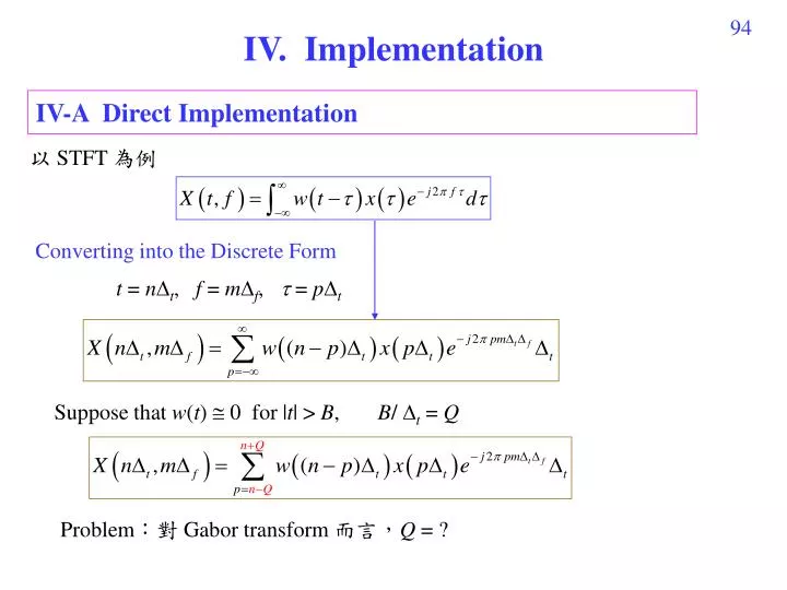
IV. Implementation. IV-A Direct Implementation. 以 STFT 為例. Converting into the Discrete Form. t = n t , f = m f , = p t. Suppose that w ( t ) 0 for | t | > B , B / t = Q. Problem :對 Gabor transform 而言, Q = ?.

E N D
IV. Implementation IV-A Direct Implementation 以 STFT 為例 Converting into the Discrete Form t = nt, f = mf, = pt Suppose that w(t) 0 for |t| > B, B/ t = Q Problem:對 Gabor transform 而言,Q = ?
Constraint for t(The only constraint for the direct implementation method) To avoid the aliasing effect, t < 1/2, is the bandwidth of ? There is no constraint for fwhen using the direct implementation method.
Four Implementation Methods (1) Direct implementation Complexity: 假設 t-axis 有 T個 sampling points, f-axis 有 F個 sampling points (2) FFT-based method Complexity: (3) FFT-based method with recursive formula Complexity: (4) Chirp-Z transform method Complexity:
IV-B FFT-Based Method Constraints: tf = 1/N, N = 1/(tf) ≧ 2Q +1: (tf 是整數的倒數) Note that the input of the FFT has less than N points (others are set to zero). Standard form of the DFT , q = p(nQ) → p = (nQ)+q where for 0 q 2Q, x1(q) = 0 for 2Q < q < N.
注意: (1) 可以使用 Matlab 的 FFT 指令來計算 (2) 對每一個 n都要計算一次
假設 t = n0t, (n0+1) t, (n0+2) t, ……, (n0+T-1)t f = m0 f, (m0+1) f, (m0+2) f, ……, (m0+F-1)f Step 1: Calculate n0, m0, T, F, N, Q Step 2: n = n0 Step 3: Determine x1(q) Step 4: X1(m) = FFT[x1(q)] Step 5: Convert X1(m) into X( nt, mf) Step 6: Set n = n+1 and return to Step 3 until n = n0+T-1. page 97
IV-C Recursive Method • A very fast way for implementing the rec-STFT • (n 和n1有recursive的關係) • (1) Calculate X(min(n)t, mf) by the N-point FFT • , n0= min(n), • for q2Q, x1(q) = 0 for q > 2Q • (2) Applying the recursive formula to calculate X(nt, mf), • n = n0 +1~ max(n) T點 F點
IV-DChirp Z Transform For the STFT Step 1 multiplication Step 2 convolution Step 3 multiplication
Step 1 n-Q p n+Q Step 2 Step 3 Step 2 在計算上,需要用到 linear convolution 的技巧 Question: Step 2 要用多少點的 DFT?
Illustration for the Question on Page 102 Case 1 When length(x[n]) = N, length( h[n]) = K, N and K are finite, length(y[n]) = N+K1, Using the (N+K1)-point DFTs (學信號處理的人一定要知道的常識) Case 2 x[n] has finite length but h[n] has infinite length ????
Case 2 x[n] has finite length but h[n] has infinite length x[n] 的範圍為 n [n1, n2],範圍大小為 N = n2− n1 + 1 h[n] 無限長 y[n] 每一點都有值 (範圍無限大) 但我們只想求出 y[n] 的其中一段 希望算出的 y[n] 的範圍為 n [m1, m2],範圍大小為 M = m2 − m1 + 1 h[n] 的範圍 ? 要用多少點的 FFT ?
改寫成 當n = m1 當n = m2
m1− n2 m1− n1 m1−n2+1 m1−n1+1 m1−n2+2 m1−n1+2 n = m1時n− s的範圍 n = m1 +1 時n− s的範圍 m2−n2 m2−n1 n = m1 +2 時n− s的範圍 n = m2時n− s的範圍 有用到的 h[k] 的範圍:k [m1− n2, m2− n1]
所以,有用到的 h[k] 的範圍是 k [m1 −n2 , m2 −n1 ] 範圍大小為 m2 − n1 − m1 + n2 + 1 = N + M − 1 FFT implementation for Case 3 for n = 0, 1, 2, … , N−1 for n = N, N + 1, N + 2, ……, L −1 L = N + M − 1 for n = 0, 1, 2, … , L−1 for n = m1, m1+1, m1+2, … , m2
IV-E Advantages and Disadvantages of the Four Methods (A) Direct Implementation Advantage: simple, flexible Disadvantage : higher complexity (B) DFT-Based Method Advantage : lower complexity Disadvantage : with some constraints (C) Recursive Method Advantage : Disadvantage : (D) Chirp Z Transform Advantage : Disadvantage :
IV-F Unbalanced Sampling for STFT and WDF 將 pages 94 and 97 的方法作修正 where t = nt, f = mf, = p, B = Q S = t/ 註:(sampling interval for the input signal) t(sampling interval for the output t-axis) can be different. However, it is better that S = t/ is an integer. (假設 w(t) 0 for |t| > B),
When (1) f= 1/N, (2) N = 1/(f) > 2Q +1: (f只要是整數的倒數即可) (3) < 1/2, is the bandwidth of i.e., when | f | > 令q = p (nSQ) → p = (nSQ) + q for 0 q 2Q, x1(q) = 0 for 2Q < q < N.
假設 t = c0t, (c0+1) t, (c0+2) t, ……, (c0+ C -1)t = c0S, (c0S+S), (c0S+2S), ……, [c0S+ (C-1)S], f = m0 f, (m0+1) f, (m0+2) f, ……, (m0+F-1)f = n0 , (n0+1) , (n0+2) , ……, (n0+T-1), S = t/ Step 1: Calculate c0, m0, n0, C, F, T, N, Q Step 2: n = c0 Step 3: Determine x1(q) Step 4: X1(m) = FFT[x1(q)w((Q-q) )] Step 5: Convert X1(m) into X( nt, mf) Step 6: Set n = n+1 and return to Step 3 until n = c0+ C -1. Complexity = ?
IV-G Non-Uniform t (A) 先用較大的t (B) 如果發現 和 之間有很大的差異 則在 nt, (n+1) t之間選用較小的 sampling interval t1 ( < t1 < t, t/ t1和t1/ 皆為整數) 再用 page 111 的方法算出 (C) 以此類推,如果 的差距還是太大,則再選用更小的 sampling interval t2 ( < t2 < t1, t1/ t2和t2/ 皆為整數)
Gabor transform of a music signal = 1/44100 (總共有 44100 1.6077 sec + 1 = 70902 點
(A) Choose t = running time = out of memory (B) Choose t = 0.01 = 441 (1.6/0.01 + 1 = 161 points) running time = 1.0940 sec (2008年) (C) Choose the sampling points on the t-axis as t = 0, 0.05, 0.1, 0.15, 0.2, 0.4, 0.45, 046, 0.47, 0.48, 0.49, 0.5, 0.55, 0.6, 0.8, 0.85, 0.9, 0.95, 0.96, 0.97, 0.98, 0.99, 1, 1.05, 1.1, 1.15, 1.2, 1.4, 1.6 (29 points) running time = 0.2970 sec
附錄四 和 Dirac Delta Function 相關的常用公式 (1) (2) (scaling property) (3) where fn are the zeros of g(f) (4) (sifting property I) (5) (sifting property II)


![Honors Level Course Implementation Guide Q & A [English I - IV]](https://cdn1.slideserve.com/3194005/honors-level-course-implementation-guide-q-a-english-i-iv-dt.jpg)