Download
1 / 7
80 likes | 225 Views
Control Charts An Introduction to Statistical Process Control. Real Life Examples. Process: Driving to Work Average Time: 12 minutes Standard Deviation: 2.5 minutes Common Causes Wind speed, miss one green light, driving speed, number of cars on road, time when leaving house, rainy weather

E N D
Control Charts An Introduction to Statistical Process Control
Real Life Examples • Process: Driving to Work • Average Time: 12 minutes • Standard Deviation: 2.5 minutes • Common Causes • Wind speed, miss one green light, driving speed, number of cars on road, time when leaving house, rainy weather • Special Causes • Stop for school bus crossing, traffic accident, pulled over for speeding, poor weather conditions, car mechanical problems, construction detour, stoplights not working properly, train crossing
Range Chart 6:55 PM45 43 48 45 50 Range = 7 UCL CL 9:35 PM44 48 43 42 45 Range = 6 LCL Range = Max of Data Subgroup – Min of Data Subgroup
How to setup EWMA chart • Determine λ (between 0 and 1) • λ is the proportion of current value used for calculating newest value • Recommend λ = 0.10, 0.20 or 0.40 (use smaller λ values to detect smaller shifts) • Calculate new z values using λ = 0.10 zi = λ*xi + (1 – λ) * zi-1 (where i = sample number) 9.7495 = (0.9*9.945) + (0.1*7.99) 9.899 = (0.9*9.7035) + (0.1*11.6)
c chart • Plots the quantity of defects in a sample • Each part can have more than one defect • Requires same number of parts within each sample 11 total defects found on 6 documents c = 11 defects per sample
Decision Tree for Control Charts What type of data: Attribute or Variable? Attribute Variable How are defects counted:Defectives (Y/N), or Count of Defects? How large are the subgroups? 1 2 to 5 5 or more Defectives Count Constant Sample Size? Constant Sample Size? X-bar and Range X-bar and Std Dev Individuals and Moving Range Yes Yes No No np chart(number defective) P chart(proportion defective) c chart(defects per sample) u chart(defects per unit)
Additional Resources Quality Management Systems Solutionshttp://www.qmss.biz