Download
1 / 29
290 likes | 401 Views
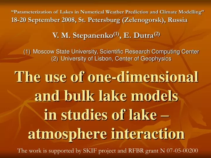
The use of one-dimensional and bulk lake models in studies of lake – atmosphere interaction. “Parameterization of Lakes in Numerical Weather Prediction and Climate Modelling” 18-20 September 2008, St. Petersburg (Zelenogorsk), Russia. V. M. Stepanenko (1) , E. Dutra (2).

E N D
The use of one-dimensionaland bulk lake models in studies of lake – atmosphere interaction “Parameterization of Lakes in Numerical Weather Prediction and Climate Modelling” 18-20 September 2008, St. Petersburg (Zelenogorsk), Russia V. M. Stepanenko(1), E. Dutra(2) • Moscow State University, Scientific Research Computing Center • University of Lisbon, Center of Geophysics The work is supported by SKIF project and RFBR grant N 07-05-00200
The effects of water reservoirs on atmosphere Weather Climate • the change of regional hydrological system due to global warming • emission of methane by Siberian lakes • breezes and associated tracer transport • severe snowfalls over large lakes in winter
Numerical water reservoir models in coupled lake – atmosphere studies • 3-dimensional (~oceanic) • 2) 2-dimensional • vertically averaged (Shlychkov) • averaged in one lateral direction (CE-QUAL x.x model) • 3) 1-dimensional • single-column (GOTM model (Burchard et al.),Lake model, V. M. Stepanenko & V. N. Lykosov, 2005); • laterally averaged models (O. F. Vasiliev et al., 2007) – applicable in many applications • 4) ½ - dimensional models – the vertical profiles of temperature, salinity etc. are parameterized (Flake model, D. V. Mironov et al., 2006) – high computational efficiency → application in operational forecast • 5) 0 – dimensional (mixed models)
Lake model (SRCC MSU) • the equation for the horizontally averaged temperature: the equations for horizontal velocities: • the salinity/hydrosol transport Coordinate transformation: • turbulent dissipation • Coriolis force • horizontal pressure gradient force • the friction of flow on vegetation • the advection by tributaries • gravitational sedimantation
Snow and soil models Ea U S Es • Ice model • Snow model (Volodina et al., 2000) • Soil model (Volodin and Lykosov, 1998) H,LE Snow Ice Water Soil (sediments) • diffusion terms • freezing terms • gravitational infiltration
Turbulent mixing parameterization - counter-gradient effects missing Kolmogorov formula (1942) M– friction frequency, N –Brunt-Vaisala frequency stability functions k-ε parameterization Boundary conditions
Willis-Deardorff experiment (1974) Setup for numerical experiment: • horizontally homogeneous water layer of infinite depth; • linear initial temperature profile with the lapse rate -1ºС/10 m; • the constant sensible heat flux at the surface 100 W/m2(cooling); • the horizontal velocities 0 m/s; • Coriolis force is neglected
The terms of turbulent energy budget 1) “E-ε” model byCanuto et al., 2001 2) LES results (Mironov et al., 2000) Lake model The k-closure The shortcoming: does not take into account non-local effects of convective thermals → does not reproduce uniform temperature profile
The counter-gradient heat transport by convective thermals (Soares et al. 2004) Temperature flux (Lake model) Temperature flux (other models and LES)
Implementation issues • Fortran 90 code • MPI libraries • Netcdf libraries • Lake driver implementation for N points (lakes) at P processors, N≥P MPI- process rank 1 k P 1 k P k Number of lake 1 k P P+1 P+k 2P 2P+k … … … … … … Number of netcdf output file k 1 P
Surface temperature from Lake model and from observations Tiksi lake, Siberia, July, 2002 Kossenblatter lake,Germany, June, 1998 Monte-Novo lake, Portugal, 1999 - 2002
The temperature in Mogaiskoe reservoir Surface temperature time series, 26.06.1996 – 13.07.1996 Vertical temperature profile, 01:00, 13.07.1996 • Important features not taken into account: • Lengmuir circulations; • Seiches; • advection by tributaries.
Snow surface temperature,(Kolpashevo, Western Siberia, February, 1961) Temperature, C Time, days
Sensible heat flux ( Flake andLake) lakeAlqueva, summer 2007
Sensible heat fluxes (Flake and Lake) Source code of Lake model and data for verification http://www.inm.ras.ru/laboratory/models_en.htm
The role of lake depth(Baikal) • The real depth - 740 m • The depth 100 m
The role of radiation extinction coefficients (Baikal and Caspian sea)
Mesoscale atmospheric model The code of Nh3d model (Miranda & James, 1992) 3-dimensional σ-coordinates non-hydrostatic equation set “warm” cloud microphysics ISBA soil model • New features: • shortwave (Clirad-SW) and longwave (Clirad-LW) radiation parameterization • lake model • aerosol transport scheme
Aerosol transport scheme - sedimentation speed, - aerosol source, - turbulent diffusion (1-st order closure), - Raileigh damping term Boundary conditions: at all boundaries • Numerical scheme:Smolarkiewich monotonous scheme • spatial discretization – 2-d order • temporal discretization – 2-d order
Aerosol distribution in test case Hanty-Mansiisk region Near surface wind • Resolution: • ∆x = ∆y = 3.7 km • 21 σ – levels • Time integration • ∆t = 5 sec • 8 days Breezes develop over water bodies and transport the tracer far from source even in calm synoptic conditions Aerosol “cloud”
The work underway: aerosol emission and sink at water bodies Aral Sea Lake Yarato lakes Norilsk: Emission of Zn, Cu, Hg,…
Future development of Lake model • Insertion the model of methane generation, transport and sink in the soil (lake sediments) – B. Walter and M. Heimann, 2000; • Introduction of the methane ebullition and bubble convection parameterization in the water body; • Incorporation of the computationally efficient version of the model into climate model of the Institute for Numerical Mathematics, Moscow; • …
Acknowledgements • Dmitrii Mikushin implemented aerosol transport scheme in mesoscale model; • Vasilii Lykosov has initiated this research and supports it; • Rui Salgado, Maria Grechushnikova provided the observational data • Pedro Soares provided the code of counter-gradient convection parameterization • Dmitrii Mironov, Pedro Viterbo, Pedro Miranda, Gianpaolo Balsamo initiated useful discussions
Thank you! Your questions are welcome!
Parallel implementation aspects Explicit scheme! FFT + Eulerian elimination Cycleswith independent iterations 1.25 % - the solution of elliptical equation for geopotential (via horizontal FFT) 2.23 % - the integration of thermodynamic equation (including radiation model) 3. 12 % - the solution of continuity equation 4.11 % - computation of turbulent transport 5.10 % - the integration of momentum equation 6.6 % - the calculation of momentum fluxes 7.5 % - the integration of water vapour and aerosol transport 8.5 % - the soil, vegetation and lake models