Download
1 / 56
560 likes | 567 Views
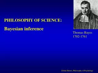
PHILOSOPHY OF SCIENCE: Neyman-Pearson approach. Jerzy Neyman April 16, 1894-August 5, 1981. Egon Pearson 11 August 1895 -12 June 1980. Zolt án Dienes, Philosophy of Psychology. 'The statistician cannot excuse himself from the duty of getting his

E N D
PHILOSOPHY OF SCIENCE: Neyman-Pearson approach Jerzy Neyman April 16, 1894-August 5, 1981 Egon Pearson 11 August 1895 -12 June 1980 Zoltán Dienes, Philosophy of Psychology
'The statistician cannot excuse himself from the duty of getting his head clear on the principles of scientific inference, but equally no other thinking person can avoid a like obligation' Fisher 1951 Much of the following material comes from Oakes, M. (1986). Statistical inference: A commentary for the social and behavioural sciences. Wiley. (out of print) If you going into research, try to get a copy!
You compare the means of a control and your experimental groups (20 subjects in each sample). The result is t(38) = 2.7, p = .01. Please mark each of the statements below as ‘true’ or ‘false’. (i) You have absolutely disproved the null hypothesis (that there is no difference between the population means). (ii) You have found the probability of the null hypothesis being true. (iii) You have absolutely proved your experimental hypothesis (that there is a difference between the population means). (iv) You can deduce the probability of the experimental hypothesis being true. (v) You know that if you decided to reject the null hypothesis, the probability that you are making the wrong decision. (vi) You have a reliable experimental finding in the sense that if, hypothetically, the experiment were repeated a great number of times, you would obtain a significant result on 99% of occasions
Probability Probabilities obey a set of axioms: P(A) ≥ 0 for an event S that always happens P(S) = 1 P(A or B) = P(A) + P(B) if A and B are mutually exclusive P(A and B) = P(A)*P(B/A) where P(B/A) is the probability of B given A But what are probabilities?
What is probability? Relative frequency interpretation Need to specify a collective of elements – like throws of a dice. Consider a case where some elements may possess property A. P(A) is the long run relative frequency of the number of elements observed having A to total number of elements observed. (In the long run – as number of observations goes to infinity – the proportion of throws of a dice showing a 3 is 1/6)
Probability is a property of a collective and not of an element in that collective: We can talk of the probability of a toss of a coin producing heads, but NOT of the probability of the 3rd toss or any particular toss doing so. This notion of probability does not apply to “the probability it will rain tomorrow” “the probability of that hypothesis being true” (The latter are examples of subjective probability – personal conviction in an opinion.)
Neyman-Pearson (defined the philosophy underlying standard statistics): Probabilities are strictly long-run relative frequencies – not subjective! If D = some data and H = a hypothesis One can talk about p(D/H) e.g. p(‘getting 5 threes in 25 rolls’/’I have a fair dice’)
Neyman-Pearson (defined the philosophy underlying standard statistics): Probabilities are strictly long-run relative frequencies – not subjective! If D = some data and H = a hypothesis One can talk about p(D/H) e.g. p(‘getting 5 threes in 25 rolls’/’I have a fair dice’) A collective or reference class we can use: the elements are ‘throwing a fair dice 25 times and observing the number of threes’ Consider a hypothetical collective of an infinite number of such elements. That is a meaningful probability we can calculate.
One can NOT talk about p(H/D) e.g. p(‘I have a fair dice’/ ‘I obtained 5 threes in 25 rolls’) What is the reference class?? The hypothesis is simply true or false.
One can NOT talk about p(H/D) e.g. p(‘I have a fair dice’/ ‘I obtained 5 threes in 25 rolls’) What is the reference class?? The hypothesis is simply true or false. P(H/D) is the inverse of the conditional probability p(D/H) Inverting conditional probabilities makes a big difference e.g. P(‘dying within two years’/’head bitten off by shark’) = 1 P(‘head was bitten off by shark’/’died in the last two years’) ~ 0 P(A/B) can have a very different value from P(B/A)
Statistics cannot tell us how much to believe a certain hypothesis. All we can do is set up decision rules for certain behaviours – accepting or rejecting hypotheses – such that in following those rules in the long run we will not often be wrong. Decision rules: Set up two contrasting hypotheses H0 the null hypothesis – the hypothesis we seek to nullify: e.g. µ1 (population mean blood pressure given drug) = µ2 (population mean blood pressure given placebo) H1: µ1 <> µ2
You collect data and summarise it as a t-value sample mean blood pressure with drug = Md sample mean blood pressure with placebo = Mp Standard error of difference = SE t = (Md – Mp)/SE Reference class: Assume H0, and imagine an infinite number of replications of the study, calculating t each time
0 t-value Distribution Work out a “rejection region” – values of t so extreme (critical value, tc) they are unlikely to occur by chance alone (say p < .05) If our obtained t is as extreme or more extreme than the critical value, we reject H0 -tc +tc
0 t-value Distribution Work out a “rejection region” – values of t so extreme (critical value, tc) they are unlikely to occur by chance alone (say p < .05) If our obtained t is as extreme or more extreme than the critical value, we reject H0 -tc +tc Put another way, we calculate p(‘getting t as extreme or more extreme than obtained’/H0) a form of P(D/H) And if the p calculated is less than level of significance we decided in advance (e.g. .05) we reject H0 By following this rule, we know in the long run that when Ho is actually true, we will conclude it false only 5% of the time
Our calculated p does not tell us how probable the null hypothesis is • it is not p(H/D) • Examples • Say you are extremely sceptical regarding ESP. • A very well controlled experiment is run on ESP giving a significant result, p =.049 ~ .05 • That does NOT mean you must now regard p(ESP exists) = 0.95. The probability of the null hypothesis is not .05. • The probability of the data given H0 is .05, but you might regard fluke a more reasonable explanation than ESP: P(D/H) does not by itself tell you how subjectively likely you think H should be.
2) I have a coin I know is biased such that p(heads) = 0.6 I throw it 6 times and it lands heads 3 times. H0: p(head) = 0.5 P(‘getting data as extreme or more extreme as 3 heads’/Ho) = 1 Non-significant! But that does not change our subjective probability that the coin is biased – we know it is biased. The probability of the coin being fair (null hypothesis) is not 1.
Our procedure tells us our long term error rates BUT it does not tell us which particular hypotheses are true or false or assign any of the hypotheses a probability. All we know is our long run error rates.
Need to control both types of error: α = p(rejecting Ho/Ho) β = p(accepting Ho/Ho false) power: P(‘getting t as extreme or more extreme than critical’/Ho false) Probability of detecting an effect given an effect really exists in the population. ( = 1 – β)
Decide on allowable α and β BEFORE you run the experiment. e.g. set α = .05 as per normal convention Ideally also set β = .05. α is just the significance level you will be testing at. But how to control β?
Decide on allowable α and β BEFORE you run the experiment. • e.g. set α = .05 as per normal convention • Ideally also set β = .05. • α is just the significance level you will be testing at. • But how to control β? • Need to • Estimate the size of effect (e.g. mean difference) you think is plausible or interesting given your theory is true • Estimate the amount of noise your data will have (e.g. typical within-group SDs of past studies) • Stats books tell you how many subjects you need to run to keep β to .05 (equivalently, to keep power at 0.95)
Most studies do not do this! But they should. Strict application of the Neyman-Pearson logic means setting the risks of both Type I and Type II errors in advance (α and β). Most researchers are extremely worried about Type I errors (false positives) but allow Type II errors (false negatives) to go uncontrolled. Leads to inappropriate judgments about what results mean and what research should be done next.
Smith and Jones, working in America, publish an experiment on a new method for reducing prejudice, with 20 subjects in each of two groups, experimental and control. They obtain a significant difference in prejudice scores between the two groups, significant by t-test, p = .02. You decide to follow up their work. Before adding modifications to their procedure, you initially attempt as exact a replication as you can in Brighton. How many subjects should you run?
Smith and Jones obtain a significant difference in prejudice scores between the two groups, significant by t-test, p = .02. Like Smith and Jones you run 20 subjects in each group. You obtain an insignificant result in the same direction, t = 1.24 (p = 0.22) Should you (a) Try to find an explanation for the difference between the two studies.
Smith and Jones obtain a significant difference in prejudice scores between the two groups, significant by t-test, p = .02. Like Smith and Jones you run 20 subjects in each group. You obtain an insignificant result in the same direction, t = 1.24 (p = 0.22) Should you (a) Try to find an explanation for the difference between the two studies. (b) Regard the Smith and Jones result as now thrown into doubt; you should reduce your confidence in the effectiveness of their method for overcoming prejudice.
Smith and Jones obtain a significant difference in prejudice scores between the two groups, significant by t-test, p = .02. Like Smith and Jones you run 20 subjects in each group. You obtain an insignificant result in the same direction, t = 1.24 (p = 0.22) Should you (a) Try to find an explanation for the difference between the two studies. (b) Regard the Smith and Jones result as now thrown into doubt; you should reduce your confidence in the effectiveness of their method for overcoming prejudice. (c) Run more subjects. (How many?)
Combining the data: t(78) = 2.59, p = .011 power N per group .67 20 .8 26 .9 37 .95 44
You read a review of studies looking at whether meditation reduces depression. 100 studies have been run and 50 are significant in the right direction and the remainder are non-significant. What should you conclude?
You read a review of studies looking at whether meditation reduces depression. 100 studies have been run and 50 are significant in the right direction and the remainder are non-significant. What should you conclude? If the null hypothesis were true, how many would be significant? How many significant in the right direction?
If your study has low power, getting a null result tells you nothing in itself. You would expect a null result whether or not the null hypothesis is true. When can you accept the null hypothesis? A null result when power is high is strong evidence that the hypothesized effect is not there.
“Even if power has been disregarded, one advantage of the .05 significance convention is that of all the significant findings in the literature, a known small proportion of them, namely 5%, are actually false rejections of the null hypothesis”
Consider a year in which of the null hypotheses we test, 4000 are actually true and 1000 actually false. Assume our power is 50%. State of World ___________________________ Decision H0 true H0 false ___________________________________________________ Accept H0 3800 500 Reject H0 200 500 ___________________________ 4000 1000 With power as low as .5, the proportion of Type I errors is not 5% but 29%! The higher the power, the less these Type I errors would be.
Why do people disregard power? 1. Because many people interpret the p value as telling them about the probability of the null (and logically hence the alternative) hypothesis. (Bayesian statisticians have developed techniques for actually assigning probabilities to hypotheses in coherent ways.) Many people interpret significance levels in a Bayesian way, and a Bayesian has no need for the concept of power. Once I know the probability of my hypothesis being true, what else do I need to know?
Why do people disregard power? 1. Because many people interpret the p value as telling them about the probability of the null (and logically hence the alternative) hypothesis. (Bayesian statisticians have developed techniques for actually assigning probabilities to hypotheses in coherent ways.) Many people interpret significance levels in a Bayesian way, and a Bayesian has no need for the concept of power. Once I know the probability of my hypothesis being true, what else do I need to know? 2. The black and white decision aspect of the Neyman-Pearson approach leads people to conclude that a effect does exist or (probably) does not. Oakes (1986)
You compare the means of a control and your experimental groups (20 subjects in each sample). The result is t(38) = 2.7, p = .01. Please mark each of the statements below as ‘true’ or ‘false’. (i) You have absolutely disproved the null hypothesis (that there is no difference between the population means). (ii) You have found the probability of the null hypothesis being true. (iii) You have absolutely proved your experimental hypothesis (that there is a difference between the population means). (iv) You can deduce the probability of the experimental hypothesis being true. (v) You know that if you decided to reject the null hypothesis, the probability that you are making the wrong decision. (vi) You have a reliable experimental finding in the sense that if, hypothetically, the experiment were repeated a great number of times, you would obtain a significant result on 99% of occasions
Further points concerning significance tests that are often misunderstood 1. Significance is a property of samples. Hypotheses are about population properties, such as means, e.g. that two means are equal or unequal. Consider the meaningless statement: “The null hypothesis states that there will be no significant difference between the conditions”. Hypothesis testing is then circular – a non-significant difference leads to the retention of the null hypothesis that there will be no significant difference! How could a significant difference between sample means ever lead to the erroneous rejection of a true null hypothesis that says there will be no significant difference! Type I errors are impossible! Dracup (1995)
2. Decision rules are laid down before data are collected; we simply make black and white decisions with known risks of error . Since significance level is decided in advance, one cannot say one result is more significant than another. Even the terms “highly significant” vs “just significant” vs “marginally significant” make no sense in the Neyman-Pearson approach. A result is significant or not, full stop.
3. A more significant result does not mean a more important result, or a larger size of effect (Is “significant” bad name? So is “reliable”.) Example of incorrect phraseology: “children in expected reward conditions solved puzzles somewhat (p < .10) faster than those in unexpected reward conditions” A large mean difference can be insignificant and a small difference significant – depending on, for example, sample size.
4. The decision rules are decided before data are collected – the significance level, sample size etc are decided in advance. Having decided on a significance level of .05, cannot then use .01 if the obtained p is e.g. .009. Similarly, having decided to run say 20 subjects, and seeing you have a not quite significant result, decide to “top up” with 10 more.
Criticism of the Neyman-Pearson approach: 1. Neyman (1938): “To decide to ‘affirm’ does not mean to ‘know’ or even ‘believe’” Is any inference involved at all? Can make no statement about the likely truth of any individual statistical hypothesis. One can talk about P(D/H) but not P(H/D) Does classic statistics evade the problem at the heart of scientific discovery?
An alternative approach is to devise techniques for calculating p(H/D) – Bayesian statistics. But remember - you need to use the specific tools of Bayesian statistics to calculate such probabilities; it is meaningless using the tools developed in the Neyman-Pearson framework.
2. In the Neyman-Pearson approach it is important to know the reference class – we must know what endless series of trials might have happened but never did.
2. In the Neyman-Pearson approach it is important to know the reference class – we must know what endless series of trials might have happened but never did. So e.g. one must distinguish planned from post hoc comparisons (Bayesian – evidential import of the data independent of the timing of the explanation)
2. In the Neyman-Pearson approach it is important to know the reference class – we must know what endless series of trials might have happened but never did. So e.g. one must distinguish planned from post hoc comparisons (Bayesian – evidential import of the data independent of the timing of the explanation) If one performed 100 significance test – if 10 significant, some unease is experienced on reflecting that if all 100 null hypotheses were true, one would expect to get 5 significant by chance alone.
2. In the Neyman-Pearson approach it is important to know the reference class – we must know what endless series of trials might have happened but never did. So e.g. one must distinguish planned from post hoc comparisons (Bayesian – evidential import of the data independent of the timing of the explanation) If one performed 100 significance test – if 10 significant, some unease is experienced on reflecting that if all 100 null hypotheses were true, one would expect to get 5 significant by chance alone. When do we correct for repeated testing? (A Bayesian does not have to) We don’t correct for all the tests we do in a paper, or for an experiment, or even in one ANOVA. Why not? Why should we correct in some cases and not others? Why should it matter what else we might have done but didn’t? Shouldn’t what actually happened be the only thing that matters?
3. Having decided on a significance level of .05, cannot then use .01 if the associated probability is e.g. .009. But is this not throwing away evidence? Can’t I get more out of my data?
4. How to take into account prior information and beliefs? One can legitimately adjust appropriate significance level – it is up to you to set α and β. Compare ESP debate – how to resolve what is the p value to use? If one just uses one judgment in an informal way, it is likely to be arbitrary and incoherent. ‘Maybe the role of subjective probability in statistics is in a sense to make statistics less subjective’ Savage et al 1962
5. Stopping rules In testing the efficacy of a drug, Psychologist A tests 20 patients and performs a t-test. It is not quite significant at the .05 level and so runs 10 more. He cannot now perform a t-test in the normal way at the .05 level (if you run until you get a significant result, you will always get a significant result). Psychologist B decides to run 30 subjects collects exactly the same data. He CAN perform a t-test at the .05 level. Should the same data lead to different conclusions because of the intentions of the experimenter? Same data lead to different conclusions. Obviously ludicrous or eminently sensible?
Neyman-Pearson: stopping rule specifies the reference class of possible outcomes by which to judge the obtained statistic. A and B wish to estimate the proportion of women in a population that have G spot orgasm. A decides in advance to sample 100 women and count the number which have G spot orgasms. He finds six which do. Best estimate of population proportion = 6/100. B decides to count women until his 6th with a G spot orgasm. That happens to be the 100th. Best estimate of population proportion = 5/99. Same data lead to different conclusions (for Bayesian both data lead to 6/100). Obviously ludicrous or eminently sensible?
6. Criticisms of null hypothesis testing a) Null hypothesis testing specifies decision rules for action (accept/reject); does not tell you how much support there is for a hypothesis.
6. Criticisms of null hypothesis testing a) Null hypothesis testing specifies decision rules for action (accept/reject); does not tell you how much support there is for a hypothesis. b) The hypothesis that m1 <> m2 or even m1 >m2 is very weak– Popper would turn in his grave. Don’t want ‘more significant’ rejections of the null hypothesis (p < .001 rather than p < .01), but more precise theories! Theorising should ultimately be more than wondering “would it make any difference if I varied this factor?”