Download
1 / 30
300 likes | 304 Views
Explore hyperspectral data of world crops from benchmark areas, including examples from USA and Central Asia. Compare hyperspectral data with other advanced sensors. Study crop separability and growth stages using hyperspectral narrowband data. Analyze hyperspectral vegetation indices of major crops.

E N D
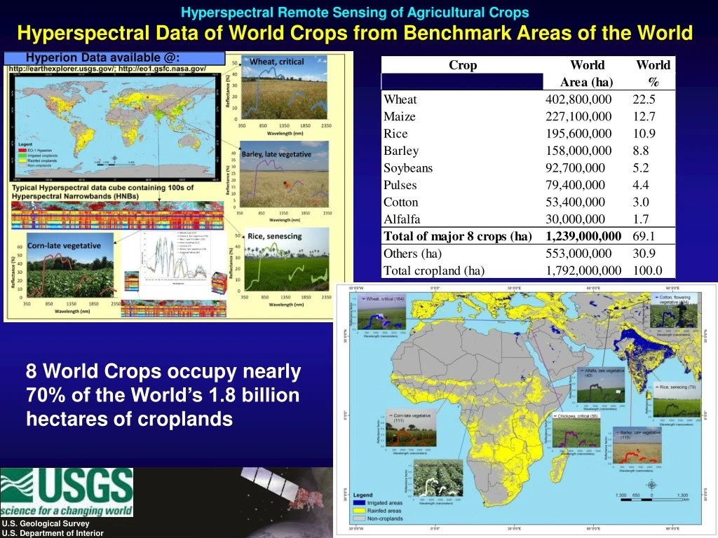
Hyperspectral Remote Sensing of Agricultural Crops Hyperspectral Data of World Crops from Benchmark Areas of the World Hyperion Data available @: 8 World Crops occupy nearly 70% of the World’s 1.8 billion hectares of croplands U.S. Geological Survey U.S. Department of Interior
Hyperspectral Remote Sensing of Agricultural Crops Hyperspectral Data of World Crops from USA Figure 3: Illustration of Hyperspectral Imaging Spectral Library of Agricultural-crops of America (HISA) of the US for 5 crops. Hyperspectral Imaging Spectral library of Agricultural crops (HISA) illustrated for 5 crops in certain agroecological zones and certain growth stages. N is number of spectra included in the average. Credits: Aneece and Thenkabail, in review U.S. Geological Survey U.S. Department of Interior
Hyperspectral Remote Sensing of Agricultural Crops Hyperspectral Data of World Crops from USA Distribution of Major crops in California used in this study Credits: Marshall and Thenkabail, 2014 U.S. Geological Survey U.S. Department of Interior
Hyperspectral Remote Sensing of Agricultural Crops Hyperspectral Data of World Crops from Central Asia Example: Cotton crop @ different Growth Stages Credit: Mariotto et al., 2013 U.S. Geological Survey U.S. Department of Interior
Hyperspectral Remote Sensing of Agricultural Crops Hyperspectral Data of World Crops from Central Asia Hyperion data of crops illustrated for typical growth stages in the Uzbekistan study area. The Hyperion data cube shown here is from a small portion of one of the two Hyperion images. The Hyperion spectra of crops are gathered from different farm fields in the two images and their average spectra illustrated here along with the sample sizes indicated within the bracket. The field data was collected within two days of the image acquisition. U.S. Geological Survey U.S. Department of Interior
Hyperspectral Remote Sensing (Imaging Spectroscopy) of Vegetation EO-1 Hyperion Pre-processing Steps Coded in Google Earth Engine U.S. Geological Survey U.S. Department of Interior Credit: Aneece et al., 2018
Comparison of Hyperspectral Data with Data from Other Advanced Sensors Hyperspectral, Hyperspatial, and Advanced Multi-spectral Data IKONOS: Feb. 5, 2002 (hyper-spatial) ETM+: March 18, 2001 (multi-spectral) ALI: Feb. 5, 2002 (multi-spectral) Hyperion: March 21, 2002 (hyper-spectral) U.S. Geological Survey U.S. Department of Interior
Comparison of Hyperspectral Data with Data from Other Advanced Sensors Hyperspectral, Hyperspatial, and Advanced Multi-spectral Data Credit:Mariotto et al., 2013 U.S. Geological Survey U.S. Department of Interior
Wheat Crop Versus Barley Crop Versus Fallow FarmHyperspectral narrowband Data for an Erectophile (65 degrees) canopy Structure wheat Barley U.S. Geological Survey U.S. Department of Interior
Wheat Crop Versus Soybean Crop Hyperspectral narrowband Data: Erectophile (65 degrees) VersusPlanophile canopy Erectophile Planophile Planophile (e.g., soybeans) Erectophile (e.g., wheat) U.S. Geological Survey U.S. Department of Interior
Hyperspectral Study of Agricultural Crops Hyperspectral Data from Various Benchmark Areas of the World for Leading World Crops Cross-site hyperspectralspectroradiometer data. Cross-site mean (regardless of which study site (1-4, Table 2)) spectral plots of eight leading world crops in various growth stages. (A) Four crops at different growth stages; (B) same four crops as in A but in different growth stages; (C) four more crops at early growth stages; and (D) same four crops as C, but at different growth stages. Note: numbers in bracket are sample sizes. U.S. Geological Survey U.S. Department of Interior
Hyperspectral Versus Multispectral Study of Agricultural Crops Hyperspectral Data from Various Benchmark Areas of the World for Leading World Crops Hyperspectral Narrowband Data Multispectral Landsat Data U.S. Geological Survey U.S. Department of Interior
Hyperspectral Narrowband Data in Study of Agricultural Crops Crop Separability in Landsat BroadbandsversusHyperspectral Narrowbands Two crop types: Hyperspectral Two crop types: Landsat Three soybean varieties Barley Wheat Galvao, L.S. et al., 2012 U.S. Geological Survey U.S. Department of Interior
Hyperspectral Remote Sensing of Agricultural Crops Linear Discriminant Analysis Corn Crop Growth Stages U.S. Geological Survey U.S. Department of Interior
Hyperspectral Vegetation Indices (HVI’s): Agricultural Crops Hyperspectral Two-band Vegetation Indices (HTBVI’s) of Hyperion Lambda versus Lambda R-square Contour plots of 2 Major Crops Contour plot of λ versus λ R2- values for wavelength bands between two-band hyperspectral vegetation indices (HVIs) and wet biomass of wheat crop (above diagonal) and corn crop (below diagonal). The 242 Hyperion bands were reduced to 157 bands after eliminating uncalibrated bands and the bands in atmospheric window. HVIs were then computed using the 157 bands leading to 12,246 unique two-band normalized difference HVIs each of which were then related to biomass to obtain R-square values. These R2-values were then plotted in a λ versus λ R2-contour plot as shown above. U.S. Geological Survey U.S. Department of Interior
Hyperspectral Vegetation Indices (HVI’s): Agricultural Crops Hyperspectral Two-band Vegetation Indices (HTBVI’s) of Hyperion Lambda versus Lambda R-square Contour plots of 2 Major Crops Contour plot of λ versus λ R2- values for wavelength bands between two-band hyperspectral vegetation indices (HVIs) and wet biomass of wheat crop (above diagonal) and corn crop (below diagonal). The 242 Hyperion bands were reduced to 157 bands after eliminating uncalibrated bands and the bands in atmospheric window. HVIs were then computed using the 157 bands leading to 12,246 unique two-band normalized difference HVIs each of which were then related to biomass to obtain R-square values. These R2-values were then plotted in a λ versus λ R2-contour plot as shown above. Credit: Mariotto et al. 2013 U.S. Geological Survey U.S. Department of Interior
Hyperspectral Vegetation Indices (HVI’s): Agricultural Crops Hyperspectral Multi-band Vegetation Indices (HMBVI’s) Best 1-band, 2-band, 3-band,…….best n-band HVI’s Note: Increase in R2 values beyond 11 bands is negligible Note: Increase in R2 values beyond 6 bands is negligible Note: Increase in R2 values beyond 17 bands is negligible U.S. Geological Survey U.S. Department of Interior
Hyperspectral Vegetation Indices (HVI’s): Agricultural Crops Hyperspectral Two-band Vegetation Indices (HTBVI’s) Multispectral Broadbands versus hyperspectral narrowbands • Note: Improved models of vegetation biophysical and biochemical variables: The combination of wavebands in Table 28.1 or HVIs derived from them provide us with significantly improved models of vegetation variables such as biomass, LAI, net primary productivity, leaf nitrogen, chlorophyll, carotenoids, and anthocyanins. For example, stepwise linear regression with a dependent plant variable (e.g., LAI, Biomass, nitrogen) and a combination of “N” independent variables (e.g., chosen by the model from Table 28.1) establish a combination of wavebands that best model a plant variable Broad-band NDVI43 vs. LAI Broad-band NDVI43 vs. WBM Narrow-band indices explain about 13 percent greater variability in modeling crop variables. Narrow-band NDVI43 vs. LAI Narrow-band NDVI43 vs. WBM U.S. Geological Survey U.S. Department of Interior
Comparison of Performance between Multispectral Broad Vegetation Indices (MVIs) VersusHyperspectral Narrowband Vegetation Indices (HVIs) California Study: Biomass Models of Major Crops (two Band VIs) • Note: • % variability explained by best models: • Rice Alfalfa Cotton Corn All • MODIS 88 61 58 10 37 • Landsat 76 82 65 53 32 • IKONOS 89 62 94 58 50 • Geoeye 88 75 95 60 55 • Worldview87 57 83 60 36 • Hyperion 92 85 98 93 71 • % 3 3 3 33 16 • Higher to totototo • In 16 27 40 83 39 • Hyperion Credit: Marshall and Thenkabail, 2014 U.S. Geological Survey U.S. Department of Interior
Comparison of Performance between Multispectral Broad Vegetation Indices (MVIs) VersusHyperspectral Narrowband Vegetation Indices (HVIs) Uzbekistan Study: Biomass models of Major Crops (Multi-linear models) • Note: • % variability explained by best models: • Cotton Corn Wheat Rice Alfalfa • ETM+ 55 62 79 N\A N\A • ALI N\A N\A N\A N\A N\ • IRS 56 73 36 N\A N\A • IKONOS 56 N\A N\A N\A N\A • Quickbird 09 N\A N\A N\A N\A • Spectro 65 96 96 100 99 • Hyperion 95 99 N\A N\A N\A • % 39 26 17 N\A N\A • Higher to tototo • In 86 37 60 N\A N\A • Hyperion • Or • Spectroradiometer Credit: Mariotto et al., 2013 U.S. Geological Survey U.S. Department of Interior
Comparison of Performance between Multispectral Broads VersusHyperspectral Narrowbands in Classification Accuracies in Classifying Crop Types • Improved accuracies in crop type classification • Hyperspectral narrowbands (HNBs) help provide significantly improved accuracies (10%–30%) in classifying Crop types compared to broadband data. U.S. Geological Survey U.S. Department of Interior
Hyperspectral Remote Sensing of Agricultural Crops Crop Type Classification Accuracies usingEO-1 Hyperion Data Crops: rice, wheat, corn, cotton, alfalfa Crops: rice, wheat, corn, cotton, soybeans Anecee and Thenkabail, in review Mariotto et al., 2013 U.S. Geological Survey U.S. Department of Interior
Hyperspectral Remote Sensing of Agricultural Crops Crop Type Classifications: corn, soybeans, cotton, rice, wheat using EO-1 Hyperion Data for USA • Improved accuracies in Crop Type Classification using various Optimal Hyperspectral Narrowbands (OHNBs) • Typically, 15-20 HNBs achieve optimal accuracies in crop type classification. In complex cases where many crops are involved upto 30 HNBs maybe required. Beyond which accuracies become asymptotic Credits: Aneece and Thenkabail, in review U.S. Geological Survey U.S. Department of Interior
Hyperspectral Remote Sensing of Agricultural Crops Crop Type Classifications: corn, soybeans, cotton, rice, wheat using EO-1 Hyperion Data for USA • Improved accuracies in Crop Type Classification using various Optimal Hyperspectral Narrowbands (OHNBs) • Typically, 15-20 HNBs achieve optimal accuracies in crop type classification. In complex cases where many crops are involved upto 30 HNBs maybe required. Beyond which accuracies become asymptotic Credits: Aneece and Thenkabail, in review U.S. Geological Survey U.S. Department of Interior
Hyperspectral Remote Sensing of Agricultural Crops Crop Type Classifications: corn, soybeans, cotton, rice, wheat using USDA CDL versus EO-1 Hyperion Data Versus for USA Original Hyperion image Hyperion using 15 OHNBs USDA CDL Hyperion using 15 OHNBs USDA CDL Original Hyperion image Overwhelmingly, 15-20 hyperspectral narrowbands (HNBs) achieved about 90% overall, producer’s, and user’s accuracies in classifying crop types and/or crop growth stages Credits:Aneece and Thenkabail, in review U.S. Geological Survey U.S. Department of Interior
Hyperspectral Remote Sensing of Agricultural Crops Selecting Targeted Optimal Hyperspectral Narrowbands (HNB’s) by Comparing Multispectral broadbands versus Hyperspectral Narrowbands U.S. Geological Survey U.S. Department of Interior
Hyperspectral Remote Sensing of Agricultural Crops References Pertaining to this Presentation Thenkabail, P.S., Mariotto, I., Gumma, M.K.,, Middleton, E.M., Landis, and D.R., Huemmrich, F.K., 2013. Selection of hyperspectralnarrowbands (HNBs) and composition of hyperspectraltwoband vegetation indices (HVIs) for biophysical characterization and discrimination of crop types using field reflectance and Hyperion/EO-1 data. IEEE JOURNAL OF SELECTED TOPICS IN APPLIED EARTH OBSERVATIONS AND REMOTE SENSING, Pp. 1-13, VOL. 6, NO. 2, APRIL 2013. U.S. Geological Survey U.S. Department of Interior
Hyperspectral Remote Sensing of Agricultural Crops Selecting Targeted Optimal Hyperspectral Narrowbands (HNB’s) byComparing Multispectral broadbands versus Hyperspectral Narrowbands Optimal hyperspectralnarrowbands (HNBs). Current state of knowledge on hyperspectralnarrowbands (HNBs) for agricultural and vegetation studies (inferred from [8]). The whole spectral analysis (WSA) using contiguous bands allow for accurate retrieval of plant biophysical and biochemical quantities using methods like continuum removal. In contrast, studies on wide array of biophysical and biochemical variables, species types, crop types have established: (a) optimal HNBs band centers and band widths for vegetation/crop characterization, (b) targeted HVIs for specific modeling, mapping, and classifying vegetation/crop types or species and parameters such as biomass, LAI, plant water, plant stress, nitrogen, lignin, and pigments, and (c) redundant bands, leading to overcoming the Hughes Phenomenon. These studies support hyperspectral data characterization and applications from missions such as Hyperspectral Infrared Imager (HyspIRI) and Advanced Responsive Tactically Effective Military Imaging Spectrometer (ARTEMIS). Note: sample sizes shown within brackets of the figure legend refer to data used in this study. Hyperspectral (Imaging Spectroscopy) Narrowband Study of Agricultural Crops Hyperspectral NarrowbandsversusMultispectral Broadbands Selecting Targeted Optimal Hyperspectral Narrowbands U.S. Geological Survey U.S. Department of Interior
Hyperspectral Remote Sensing of Agricultural Crops References Pertaining to this Presentation • 1. Thenkabail, P.S., 2015. Hyperspectral Remote Sensing for Terrestrial Applications. Chapter 9, In Thenkabail, P.S., (Editor-in-Chief), 2015. “Remote Sensing Handbook” Volume II: Land Resources: Monitoring, Modeling, and Mapping: Advances over Last 50 Years and a Vision for the Future,Book Chapter. Taylor and Francis Inc.\CRC Press, Boca Raton, London, New York. Pp. 800+. In Press (planned publication in November, 2015). • 2. Thenkabail, P.S., Mariotto, I., Gumma, M.K.,, Middleton, E.M., Landis, and D.R., Huemmrich, F.K., 2013. Selection of hyperspectral narrowbands (HNBs) and composition of hyperspectral twoband vegetation indices (HVIs) for biophysical characterization and discrimination of crop types using field reflectance and Hyperion/EO-1 data. IEEE JOURNAL OF SELECTED TOPICS IN APPLIED EARTH OBSERVATIONS AND REMOTE SENSING, Pp. 427-439, VOL. 6, NO. 2, APRIL 2013.doi: 10.1109/JSTARS.2013.2252601 • 3. Marshall M. T., and Thenkabail P. 2015. Developing in situ Non-Destructive Estimates of Crop Biomass to Address Issues of Scale in Remote Sensing.Remote Sensing. 2015; 7(1):808-835. doi:10.3390/rs70100808 • 4. Marshall, M.T., Thenkabail, P.S. 2014. Biomass modeling of four leading World crops using hyperspectral narrowbands in support of HyspIRI mission.Photogrammetric Engineering and Remote Sensing. 80(4): 757-772. • 5. Mariotto, I., Thenkabail, P.S., Huete, H., Slonecker, T., Platonov, A., 2013. Hyperspectral versus Multispectral Crop- Biophysical Modeling and Type Discrimination for the HyspIRI Mission.Remote Sensing of Environment. 139:291-305 U.S. Geological Survey U.S. Department of Interior
Hyperspectral Remote Sensing of Agricultural Crops References Pertaining to this Presentation 6. Thenkabail, P.S., Enclona, E.A., Ashton, M.S., Legg, C., Jean De Dieu, M., 2004. Hyperion, IKONOS, ALI, and ETM+ sensors in the study of African rainforests. Remote Sensing of Environment, 90:23-43. 7. Thenkabail, P.S., Enclona, E.A., Ashton, M.S., and Van Der Meer, V. 2004. Accuracy Assessments of Hyperspectral Waveband Performance for Vegetation Analysis Applications. Remote Sensing of Environment, 91:2-3: 354-376. 8. Thenkabail, P.S. 2003. Biophysical and yield information for precision farming from near-real time and historical Landsat TM images. International Journal of Remote Sensing. 24(14): 2879-2904. 9. Thenkabail P.S., Smith, R.B., and De-Pauw, E. 2002. Evaluation of Narrowband and Broadband Vegetation Indices for Determining Optimal Hyperspectral Wavebands for Agricultural Crop Characterization. Photogrammetric Engineering and Remote Sensing. 68(6): 607-621. 10. Thenkabail, P.S., 2002. Optimal HyperspectralNarrowbands for Discriminating Agricultural Crops. Remote Sensing Reviews. 20(4): 257-291. 11. Thenkabail P.S., Smith, R.B., and De-Pauw, E. 2000b. Hyperspectral vegetation indices for determining agricultural crop characteristics. Remote sensing of Environment. 71:158-182. 12. Thenkabail P.S., Smith, R.B., and De-Pauw, E. 1999. Hyperspectral vegetation indices for determining agricultural crop characteristics. CEO research publication series No. 1, Center for earth Observation, Yale University. Pp. 47. Monograph\Book:ISBN:0-9671303-0-1. (Yale University, New Haven). U.S. Geological Survey U.S. Department of Interior