Numerical Integration Formulas

1. Numerical Integration Formulas Berlin Chen Department of Computer Science & Information Engineering National Taiwan Normal University Reference: 1. Applied Numerical Methods with MATLAB for Engineers, Chapter 19 & Teaching material

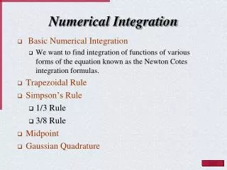
2. Chapter Objectives (1/2) • Recognizing that Newton-Cotes integration formulas are based on the strategy of replacing a complicated function or tabulated data with a polynomial that is easy to integrate • Knowing how to implement the following single application Newton-Cotes formulas: • Trapezoidal rule • Simpson’s 1/3 rule • Simpson’s 3/8 rule • Knowing how to implement the following composite Newton-Cotes formulas: • Trapezoidal rule • Simpson’s 1/3 rule

3. Chapter Objectives (2/2) • Recognizing that even-segment-odd-point formulas like Simpson’s 1/3 rule achieve higher than expected accuracy • Knowing how to use the trapezoidal rule to integrate unequally spaced data • Understanding the difference between open and closed integration formulas

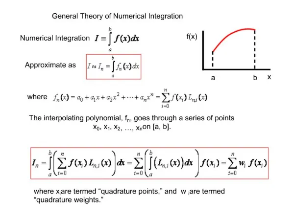
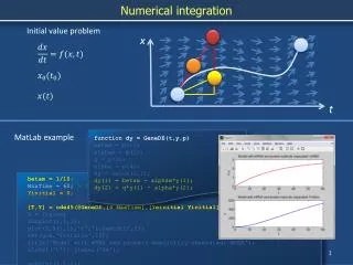
4. Integration • Integration: is the total value, or summation, of f(x) dx over the range from a to b:

5. Newton-Cotes Formulas • The Newton-Cotes formulas are the most common numerical integration schemes • Generally, they are based on replacing a complicated function or tabulated data with a polynomial that is easy to integrate: • where fn(x) is an nth order interpolating polynomial

6. Newton-Cotes Examples • The integrating function can be polynomials for any order - for example, (a) straight lines or (b) parabolas • The integral can be approximated in one step or in a series of steps to improve accuracy

7. The Trapezoidal Rule • The trapezoidal ruleis the first of the Newton-Cotes closed integration formulas; it uses a straight-line approximation for the function:

8. Error of the Trapezoidal Rule • An estimate for the local truncation error of a single application of the trapezoidal rule is:where is somewhere between a and b • This formula indicates that the error is dependent upon the curvature of the actual function as well as the distance between the points • Error can thus be reduced by breaking the curve into parts

9. Trapezoidal Rule: An Example Example 19.1

10. Composite Trapezoidal Rule • Assuming n+1 data points are evenly spaced, there will be n intervals over which to integrate • The total integral can be calculated by integrating each subinterval and then adding them together:

11. Composite Trapezoidal Rule: An Example Example 19.2

12. MATLAB Program

13. Simpson’s Rules • One drawback of the trapezoidal rule is that the error is related to the second derivative of the function • More complicated approximation formulas can improve the accuracy for curves - these include using (a) 2nd and (b) 3rd order polynomials • The formulas that result from taking the integrals under these polynomials are called Simpson’s rules

14. Simpson’s 1/3 Rule • Simpson’s 1/3 rule corresponds to using second-order polynomials. Using the Lagrange form for a quadratic fit of three points: • Integration over the three points simplifies to:

15. Error of Simpson’s 1/3 Rule • An estimate for the local truncation error of a single application of Simpson’s 1/3 rule is:where again is somewhere between a and b • This formula indicates that the error is dependent upon the fourth-derivative of the actual function as well as the distance between the points • Note that the error is dependent on the fifth power of the step size (rather than the third for the trapezoidal rule) • Error can thus be reduced by breaking the curve into parts

16. Simpson’s 1/3 Rule: An Example Example 19.3

17. Composite Simpson’s 1/3 Rule • Simpson’s 1/3 rule can be used on a set of subintervals in much the same way the trapezoidal rule was, except there must be an odd number of points • Because of the heavy weighting of the internal points, the formula is a little more complicated than for the trapezoidal rule:

18. Composite Simpson’s 1/3 Rule: An Example Example 19.4

19. Simpson’s 3/8 Rule • Simpson’s 3/8 rule corresponds to using third-order polynomials to fit four points. Integration over the four points simplifies to: • Simpson’s 3/8 rule is generally used in concert with Simpson’s 1/3 rule when the number of segments is odd

20. Simpson’s 3/8 Rule: An Example (1/2) Example 19.5

21. Simpson’s 3/8 Rule: An Example (2/2)

22. Higher-Order Formulas • Higher-order Newton-Cotes formulas may also be used - in general, the higher the order of the polynomial used, the higher the derivative of the function in the error estimate and the higher the power of the step size • As in Simpson’s 1/3 and 3/8 rule, the even-segment-odd-point formulas have truncation errors that are the same order as formulas adding one more point. For this reason, the even-segment-odd-point formulas are usually the methods of preference

23. Integration with Unequal Segments • Previous formulas were simplified based on equispaced data points - though this is not always the case • The trapezoidal rule may be used with data containing unequal segments:

24. Integration Code for Unequal Segments

25. MATLAB Functions • MATLAB has built-in functions to evaluate integrals based on the trapezoidal rule • z = trapz(y)z = trapz(x, y)produces the integral of y with respect to x. If x is omitted, the program assumes h=1 • z = cumtrapz(y)z = cumtrapz(x, y)produces the cumulative integral of y with respect to x. If x is omitted, the program assumes h=1

26. Multiple Integrals • Multiple integrals can be determined numerically by first integrating in one dimension, then a second, and so on for all dimensions of the problem