Download
1 / 17
310 likes | 858 Views
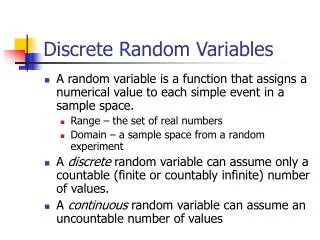
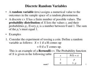
12.5 – The Normal Distribution. Discrete and Continuous Random Variables. Discrete random variable: A random variable that can take on only certain fixed values. The number of even values of a single die. The number of heads in three tosses of a fair coin.

E N D
12.5 – The Normal Distribution Discrete and Continuous Random Variables Discrete random variable: A random variable that can take on only certain fixed values. The number of even values of a single die. The number of heads in three tosses of a fair coin. Continuous random variable: A variable whose values are not restricted. The diameter of a growing tree. The height of third graders.
12.5 – The Normal Distribution Definition and Properties of a Normal Curve A normal curve is a symmetric, bell-shaped curve. Any random continuous variable whose graph has this characteristic shape is said to have a normal distribution. On a normal curve the horizontal axis is labeled with the mean and the specific data values of the standard deviations. If the horizontal axis is labeled using the number of standard deviations from the mean, rather than the specific data values, then the curve the standard normal curve
12.5 – The Normal Distribution Sample Statistics Normal Curve Standard Normal Curve 1 2 1.4 – 1 2.8 – 2 – 2.8 – 1.4 0 or 5.5 5.5
12.5 – The Normal Distribution Normal Curves B S A C 0 S is standard, with mean = 0, standard deviation = 1 A has mean < 0, standard deviation = 1 B has mean = 0, standard deviation < 1 C has mean > 0, standard deviation > 1
12.5 – The Normal Distribution Properties of Normal Curves The graph of a normal curve is bell-shaped and symmetric about a vertical line through its center. The mean, median, and mode of a normal curve are all equal and occur at the center of the distribution. Empirical Rule: the approximate percentage of all data lying within 1, 2, and 3 standard deviations of the mean. within 1 standard deviation 68% within 2 standard deviations 95% within 3 standard deviations. 99.7%
12.5 – The Normal Distribution Empirical Rule 68% 95% 99.7%
12.5 – The Normal Distribution Example: Applying the Empirical Rule A sociology class of 280 students takes an exam. The distribution of their scores can be treated as normal. Find the number of scores falling within 2 standard deviations of the mean. A total of 95% of all scores lie within 2 standard deviations of the mean. (.95)(280) = 266 scores
12.5 – The Normal Distribution Normal Curve Areas In a normal curve and a standard normal curve, the total area under the curve is equal to 1. The area under the curve is presented as one of the following: • Percentage (of total items that lie in an interval), • Probability (of a randomly chosen item lying in an interval), • Area (under the normal curve along an interval).
12.5 – The Normal Distribution A Table of Standard Normal Curve Areas To answer questions that involve regions other than 1, 2, or 3 standard deviations, a Table of Standard Normal Curve Areas is necessary. The table shows the area under the curve for all values in a normal distribution that lie between the mean and z standard deviations from the mean. The percentage of values within a certain range of z-scores, or the probability of a value occurring within that range are the more common uses of the table. Because of the symmetry of the normal curve, the table can be used for values above the mean or below the mean.
12.5 – The Normal Distribution Example: Applying the Normal Curve Table Use the table to find the percent of all scores that lie between the mean and 1.5 standard deviations above the mean. z = 1.5 Find 1.50 in the z column. The table entry is .4332 z = 1.50 Therefore, 43.32% of all values lie between the mean and 1.5 standard deviations above the mean. or There is a .4332 probability that a randomly selected value will lie between the mean and 1.5 standard deviations above the mean.
12.5 – The Normal Distribution Example: Applying the Normal Curve Table Use the table to find the percent of all scores that lie between the mean and 2.62 standard deviations below the mean. z = –2.62 The table entry is 0.4956 z = – 2.62 Find 2.62 in the z column. Therefore, 49.56% of all values lie between the mean and 2.62 standard deviations below the mean. or There is a 0.4956 probability that a randomly selected value will lie between the mean and 2.62 standard deviations below the mean.
12.5 – The Normal Distribution Example: Applying the Normal Curve Table Find the percent of all scores that lie between the given z-scores. z = –1.7 z = 2.55 z = – 1.7 The table entry is 0.4554 z = 2.55 The table entry is 0.4946 0.4554 + 0.4946 = 0.95 Therefore, 95% of all values lie between – 1.7 and 2.55 standard deviations.
12.5 – The Normal Distribution Example: Applying the Normal Curve Table Find the probability that a randomly selected value will lie between the given z-scores. z = 0.61 z = 2.63 z = 0.61 The table entry is 0.2291 z = 2.63 The table entry is 0.4957 0.4957 – 0.2291 = 0.2666 There is a 0.2666 probability that a randomly selected value will lie between 0.61 and 2.63 standard deviations.
12.5 – The Normal Distribution Example: Applying the Normal Curve Table Find the probability that a randomly selected value will lie above the given z-score. z = 2.14 z = 2.14 The table entry is 0.4838 Half of the area under the curve is 0.5000 0.5000 – 0.4838 = 0.0162 There is a 0.0162 probability that a randomly selected value will lie 2.14 standard deviations.
12.5 – The Normal Distribution Example: Applying the Normal Curve Table The volumes of soda in bottles from a small company are distributed normally with a mean of 12 ounces and a standard deviation .15 ounces. If 1 bottle is randomly selected, what is the probability that it will have more than 12.33 ounces? z = 2.2 The table entry is 0.4861 12.33 Half of the area under the curve is 0.5000 0.5000 – 0.4861 = 0.0139 There is a 0.0139 probability that a randomly selected bottle will contain more than 12.33 ounces.
12.5 – The Normal Distribution Example: Finding z-scores for Given Areas Assuming a normal distribution, find the z-score meeting the condition that 39% of the area is to the right of z. 50% of the area lies to the right of the mean. = 0.11 11% The areas from the Normal Curve Table are based on the area between the mean and the z-score. = 0.39 39% area between the mean and the z-score = 0.50 – 0.39 = 0.11 From the table, find the area of 0.1100 or the closest value and read the z-score. z-score = 0.28
12.5 – The Normal Distribution Example: Finding z-scores for Given Areas Assuming a normal distribution, find the z-score meeting the condition that 76% of the area is to the left of z. 50% of the area lies to the left of the mean. 26% = 0.26 50% The areas from the Normal Curve Table are based on the area between the mean and the z-score. 0.5000 area between the mean and the z-score = 0.76 – 0.50 = 0.26 From the table, find the area of 0.2600 or the closest value and read the z-score. z-score = 0.71