Download
1 / 21
220 likes | 256 Views
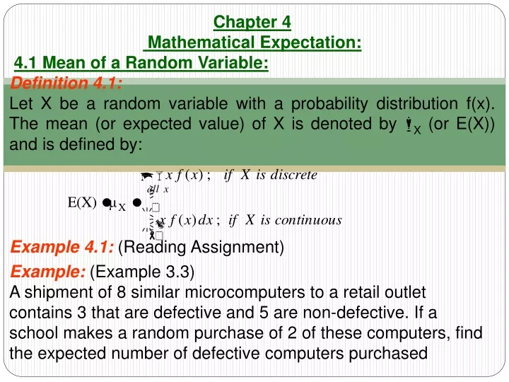
Chapter 4 Mathematical Expectation: 4.1 Mean of a Random Variable: Definition 4.1: Let X be a random variable with a probability distribution f(x). The mean (or expected value) of X is denoted by X (or E(X)) and is defined by:. Example 4.1: (Reading Assignment). Example: (Example 3.3)

E N D
Chapter 4 Mathematical Expectation: 4.1 Mean of a Random Variable: Definition 4.1: Let X be a random variable with a probability distribution f(x). The mean (or expected value) of X is denoted by X (or E(X)) and is defined by: Example 4.1: (Reading Assignment) Example:(Example 3.3) A shipment of 8 similar microcomputers to a retail outlet contains 3 that are defective and 5 are non-defective. If a school makes a random purchase of 2 of these computers, find the expected number of defective computers purchased
Solution: Let X = the number of defective computers purchased. In Example 3.3, we found that the probability distribution of X is: or:
The expected value of the number of defective computers purchased is the mean (or the expected value) of X, which is: = (0) f(0) + (1) f(1) +(2) f(2) (computers) Example 4.3: Let X be a continuous random variable that represents the life (in hours) of a certain electronic device. The pdf of X is given by: Find the expected life of this type of devices.
(hours) Solution: Therefore, we expect that this type of electronic devices to last, on average, 200 hours.
Theorem 4.1: Let X be a random variable with a probability distribution f(x), and let g(X) be a function of the random variable X. The mean (or expected value) of the random variable g(X) is denoted by g(X) (or E[g(X)]) and is defined by: Example: Let X be a discrete random variable with the following probability distribution Find E[g(X)], where g(X)=(X 1)2.
Solution: g(X)=(X 1)2 = (01)2 f(0) + (11)2 f(1) +(21)2 f(2) = (1)2 + (0)2 +(1)2
Example: In Example 4.3, find E . Solution:
4.2 Variance (of a Random Variable): The most important measure of variability of a random variable X is called the variance of X and is denoted by Var(X) or . Definition: The positive square root of the variance of X, ,is called the standard deviation of X. Definition 4.3: Let X be a random variable with a probability distribution f(x) and mean . The variance of X is defined by: Note: Var(X)=E[g(X)], where g(X)=(X )2
Theorem 4.2: The variance of the random variable X is given by: where Find Var(X)= . Example 4.9: Let X be a discrete random variable with the following probability distribution
Solution: = (0) f(0) + (1) f(1) +(2) f(2) + (3) f(3) = (0) (0.51) + (1) (0.38) +(2) (0.10) + (3) (0.01) = 0.61 1. First method: =(00.61)2 f(0)+(10.61)2 f(1)+(20.61)2 f(2)+ (30.61)2 f(3) =(0.61)2 (0.51)+(0.39)2 (0.38)+(1.39)2 (0.10)+ (2.39)2 (0.01) = 0.4979 2. Second method: = (02) f(0) + (12) f(1) +(22) f(2) + (32) f(3) = (0) (0.51) + (1) (0.38) +(4) (0.10) + (9) (0.01) = 0.87 =0.87 (0.61)2 = 0.4979
Example 4.10: Let X be a continuous random variable with the following pdf: Find the mean and the variance of X. Solution: 5/3 17/6 17/6 – (5/3)2 = 1/8
4.3 Means and Variances of Linear Combinations of Random Variables: If X1, X2, …, Xn are n random variables and a1, a2, …, an are constants, then the random variable : is called a linear combination of the random variables X1,X2,…,Xn. Theorem 4.5: If X is a random variable with mean =E(X), and if aand b are constants, then: E(aXb) = a E(X) b aXb = a X ± b Corollary 1:E(b) = b (a=0 in Theorem 4.5) Corollary 2: E(aX) = a E(X) (b=0 in Theorem 4.5)
Example 4.16: Let X be a random variable with the following probability density function: Find E(4X+3). Solution: 5/4 E(4X+3) = 4 E(X)+3 = 4(5/4) + 3=8 Another solution: ; g(X) = 4X+3 E(4X+3) =
Theorem: If X1, X2, …, Xn are n random variables and a1, a2, …, an are constants, then: E(a1X1+a2X2+ … +anXn) = a1E(X1)+ a2E(X2)+ …+anE(Xn) Theorem 4.9: If X is a random variable with variance and if aand b are constants, then: Var(aXb) = a2 Var(X) Corollary: If X, and Y are random variables, then: E(X± Y) = E(X) ± E(Y)
Theorem: If X1, X2, …, Xn are n independent random variables and a1, a2, …, an are constants, then: Var(a1X1+a2X2+…+anXn) = Var(X1)+ Var (X2)+…+ Var(Xn) Corollary: If X, and Y are independent random variables, then: · Var(aX+bY) = a2 Var(X) + b2 Var (Y) · Var(aXbY) = a2 Var(X) + b2 Var (Y) · Var(X ± Y) = Var(X) + Var (Y)
Example: Let X, and Y be two independent random variables such that E(X)=2, Var(X)=4, E(Y)=7, and Var(Y)=1. Find: 1. E(3X+7) and Var(3X+7) 2. E(5X+2Y2) and Var(5X+2Y2). Solution: 1. E(3X+7) = 3E(X)+7 = 3(2)+7 = 13 Var(3X+7)= (3)2 Var(X)=(3)2 (4) =36 2. E(5X+2Y2)= 5E(X) + 2E(Y) 2= (5)(2) + (2)(7) 2= 22 Var(5X+2Y2)= Var(5X+2Y)= 52 Var(X) + 22 Var(Y) = (25)(4)+(4)(1) = 104
4.4 Chebyshev's Theorem: * Suppose that X is any random variable with mean E(X)= and variance Var(X)= and standard deviation . * Chebyshev's Theorem gives a conservative estimate of the probability that the random variable X assumes a value within k standard deviations (k) of its mean , which is P( k <X< +k). * P( k <X< +k) 1
Theorem 4.11:(Chebyshev's Theorem) Let X be a random variable with mean E(X)= and variance Var(X)=2, then for k>1, we have: P( k <X< +k) 1 P(|X | < k) 1 Example 4.22: Let X be a random variable having an unknown distribution with mean =8 and variance 2=9 (standard deviation =3). Find the following probability: (a) P(4 <X< 20) (b) P(|X8| 6)
Solution: (a) P(4 <X< 20)= ?? P( k <X< +k) 1 (4 <X< 20)= ( k <X< +k) 4= k 4= 8 k(3) or 20= + k 20= 8+ k(3) 4= 8 3k 20= 8+ 3k 3k=12 3k=12 k=4 k=4 Therefore, P(4 <X< 20) , and hence,P(4 <X< 20) (approximately)
(b) P(|X 8| 6)= ?? P(|X8| 6)=1 P(|X8| < 6) P(|X 8| < 6)= ?? P(|X | < k) 1 (|X8| < 6) = (|X | < k) 6= k 6=3k k=2 P(|X8| < 6) 1 P(|X8| < 6) 1 1 P(|X8| < 6) P(|X8| 6) Therefore, P(|X8| 6) (approximately)
Another solution for part (b): P(|X8| < 6) = P(6 <X8 < 6) = P(6 +8<X < 6+8) = P(2<X < 14) (2<X <14) = ( k <X< +k) 2= k 2= 8 k(3) 2= 8 3k 3k=6 k=2 P(2<X < 14) P(|X8| < 6) 1 P(|X8| < 6) 1 1 P(|X8| < 6) P(|X8| 6) Therefore, P(|X8| 6) (approximately)