Download
1 / 72
720 likes | 732 Views
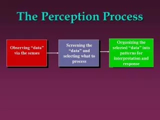
The Perception Processor. Binu Mathew Advisor: Al Davis. What is Perception Processing ?. Ubiquitous computing needs natural human interfaces Processor support for perceptual applications Gesture recognition Object detection, recognition, tracking Speech recognition

E N D
The Perception Processor Binu Mathew Advisor: Al Davis
What is Perception Processing ? • Ubiquitous computing needs natural human interfaces • Processor support for perceptual applications • Gesture recognition • Object detection, recognition, tracking • Speech recognition • Speaker identification • Applications • Multi-modal human friendly interfaces • Intelligent digital assistants • Robotics, unmanned vehicles • Perception prosthetics
The Problem with Perception Processing • Too slow, too much power for embedded space! • 2.4 GHz Pentium 4 ~ 60 Watts • 400 MHz Xscale ~ 800 mW • 10x or more difference in performance • Inadequate memory bandwidth • Sphinx requires 1.2 GB/s memory bandwidth • Xscale delivers 64 MB/s ~ 1/19th • Characterize application to find the problem • Derive acceleration architecture • History of FPUs is an analogy
High Level Architecture Processor Coprocessor Interface Memory Controller Input SRAMs Custom Accelerator Output SRAM DRAM Interface Scratch SRAMS
Thesis Statement It is possible to design programmable processors that can handle sophisticated perception workloads in real-time at power budgets suitable for embedded devices.
FaceRec In Action Rob Evans
Application Structure Rowley Face Detector • Flesh toning: Soriano et al, Bertran et al • Segmentation: Text book approach • Rowley detector, voter: Henry Rowley, CMU • Viola & Jones’ detector: Published algorithm + Carbonetto, UBC • Eigenfaces: Re-implementation by Colorado State University Neural Net Eye Locator Eigenfaces Face Recognizer Segment Image Flesh tone Image Viola & Jones Face Detector Identity, Coordinates
FaceRec Characterization • ML-RSIM out of order processor simulator • SPARC V8 ISA, Unmodified SunOS binaries
Why is IPC low ? Neural Network Evaluation: Sum = Σn i=0 Weight[i] * Image[ Input[i] ] Result = Tanh(Sum) • Dependences – e.g.: no single cycle floating point accumulate • Indirect accesses • Several array accesses per operator • Load store ports saturate • Need architectures that can move data efficiently
Example App: CMU Sphinx 3.2 • Speech recognition engine • Speaker and language independent • Acoustic model: Triphone based, continuous • Hidden Markov Model (HMM) based • Grammar: Trigram with back-off • Open source HUB4 speech model • Broadcast news model (ABC news, NPR etc) • 64000 word vocabulary
High Level Architecture Processor Coprocessor Interface Memory Controller Input SRAMs Custom Accelerator Output SRAM DRAM Interface Scratch SRAMS
ASIC Accelerator Design: Matrix Multiply def matrix_multiply(A, B, C): # C is the result matrix for i in range(0, 16): for j in range(0, 16): C[i][j] = inner_product(A, B, i, j) def inner_product(A, B, row, col): sum = 0.0 for i in range(0,16): sum = sum + A[row][i] * B[i][col] return sum
ASIC Accelerator Design: Matrix Multiply Control Pattern def matrix_multiply(A, B, C): # C is the result matrix for i in range(0, 16): for j in range(0, 16): C[i][j] = inner_product(A, B, i, j) def inner_product(A, B, row, col): sum = 0.0 for i in range(0,16): sum = sum + A[row][i] * B[i][col] return sum
ASIC Accelerator Design: Matrix Multiply Access Pattern def matrix_multiply(A, B, C): # C is the result matrix for i in range(0, 16): for j in range(0, 16): C[i][j] = inner_product(A, B, i, j) def inner_product(A, B, row, col): sum = 0.0 for i in range(0,16): sum = sum + A[row][i] * B[i][col] return sum
ASIC Accelerator Design: Matrix Multiply Compute Pattern def matrix_multiply(A, B, C): # C is the result matrix for i in range(0, 16): for j in range(0, 16): C[i][j] = inner_product(A, B, i, j) def inner_product(A, B, row, col): sum = 0.0 for i in range(0,16): sum = sum + A[row][i] * B[i][col] return sum
ASIC Accelerator Design: Matrix Multiply def matrix_multiply(A, B, C): # C is the result matrix for i in range(0, 16): for j in range(0, 16): C[i][j] = inner_product(A, B, i, j) def inner_product(A, B, row, col): sum = 0.0 for i in range(0,16): sum = sum + A[row][i] * B[i][col] return sum
ASIC Accelerator Design: Matrix Multiply 7 cycle latency def matrix_multiply(A, B, C): # C is the result matrix for i in range(0, 16): for j in range(0, 16): C[i][j] = inner_product(A, B, i, j) def inner_product(A, B, row, col): sum = 0.0 for i in range(0,16): sum = sum + A[row][i] * B[i][col] return sum
ASIC Accelerator Design: Matrix Multiply Interleave >= 7 inner products Complicates address generation def matrix_multiply(A, B, C): # C is the result matrix for i in range(0, 16): for j in range(0, 16): C[i][j] = inner_product(A, B, i, j) def inner_product(A, B, row, col): sum = 0.0 for i in range(0,16): sum = sum + A[row][i] * B[i][col] return sum
How can we generalize ? • Decompose loop into: • Control pattern • Access pattern • Compute pattern Programmable h/w acceleration for each pattern
Address Generator A[(i+k1)<<k2+k3][(j+k4)<<k5+k6] A[B[i]]
Inner Product Micro-code i_loop = LoopContext(start_count=0, end_count=15, increment=1, II=7 ) A_ri = AddressContext(port=inq.a_port, loop0=row_loop, rowsize=16, loop1=i_loop, base=0) B_ic = AddressContext(port=inq.b_port, loop0=i_loop, rowsize=16, loop1=Constant, base=256) for i in LOOP(i_loop): t0 = LOAD( fpu0.a_reg, A_ri ) for k in range(0,7): # Will be unrolled 7x AT(t0 + k) t1 = LOAD(fpu0.b_reg, B_ic, loop1_constant=k) AT(t1) t2 = fpu0.mult( fpu0.a_reg, fpu0.b_reg ) AT(t2) t3 = TRANSFER( fpu1.b_reg, fpu0 ) AT(t3) fpu1.add( fpu1, fpu1.b_reg )
Modulo Scheduling - Problem i, j i+1, j i+2, j i+3, j
Traditional Solution • Generate multiple copies of address calculation instructions • Use register rotation to fix dependences
Traditional Solution • Generate multiple copies of address calculation instructions • Use register rotation to fix dependences
Array Variable Renaming tag=0 tag=1 tag=2 tag=3
Experimental Method • Measure processor power on • 2.4 GHz Pentium 4, 0.13u process • 400 MHz XScale, 0.18u process • Perception Processor • 1 GHz, 0.13u process (Berkeley Predictive Tech Model) • Verilog, MCL HDLs • Synthesized using Synopsys Design Compiler • Fanout based heuristic wire loads • Spice (Nanosim) simulation yields current waveform • Numerical integration to calculate energy • ASICs in 0.25u process • Normalize 0.18u, 0.25u energy and delay numbers
Benchmarks • Visual feature recognition • Erode, Dilate: Image segmentation opertators • Fleshtone: NCC flesh tone detector • Viola, Rowley: Face detectors • Speech recognition • HMM: 5 state Hidden Markov Model • GAU: 39 element, 8 mixture Gaussian • DSP • FFT: 128 point, complex to complex, floating point • FIR: 32 tap, integer • Encryption • Rijndael: 128 bit key, 576 byte packets
Results: IPC Mean IPC = 3.3x R14K