Download
1 / 65
650 likes | 652 Views
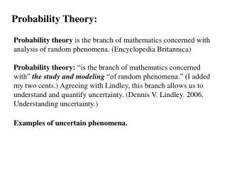
Probability theory retro. 14/03/2017. Probability. (atomic) events (A) and probability space ( ) Axioms: - 0 ≤ P(A) ≤ 1 - P( )=1 - If A 1 , A 2 , … mutually exclusive events (A i ∩A j = , i j ) then P( k A k ) = k P( A k ). 1. - P( Ø ) = 0 - P( ¬ A)=1-P(A)

E N D
Probability theoryretro 14/03/2017
Probability (atomic) events (A) and probability space () Axioms: - 0 ≤ P(A) ≤ 1 - P()=1 - If A1, A2, … mutually exclusive events (Ai ∩Aj = , i j) then P(k Ak) = k P(Ak) 1
- P(Ø) = 0 - P(¬A)=1-P(A) - P(A B)=P(A)+P(B) – P(A∩B) - P(A) = P(A ∩ B)+P(A ∩¬B) If A B, then P(A) ≤ P(B) and P(B-A) = P(B) – P(A) 2
Conditional probability Conditional probability is the probability of some event A, given the occurrence of some other event B. P(A|B) = P(A∩B)/P(B) Chain rule: P(A∩B) = P(A|B)·P(B) Example: A: headache, B: influenza P(A) = 1/10, P(B) = 1/40, P(A|B)=? 3
Independence of events A and B are independent iff P(A|B) = P(A) Corollary: P(AB) = P(A)P(B) P(B|A) = P(B) 5
Product rule A1, A2, …, An arbitrary events P(A1A2…An) = P(An|A1…An-1) P(An-1|A1…An-2)…P(A2| A1)P(A1) If A1, A2, …, An events form a complete probability space and P(Ai) > 0 for each i, then P(B) = ∑j=1nP(B |Ai)P(Ai) 6
Bayes rule P(A|B) = P(A∩B)/P(B) = P(B|A)P(A)/P(B) 7
Random variable ξ: → R Random variable vectors… 8
cumulative distribution function (CDF), F(x) = P( < x) F(x1) ≤ F(x2), if x1 < x2 limx→-∞F(x) = 0, limx→∞F(x) = 1 F(x) is non-decreasing and right-continuous 9
Discrete vs continousrandom variables Discrete: its value set forms a finite of infinate series Continous: we assume that f(x) is valid on the (a, b) interval 10
Probabilitydensityfunctions (pdf) F(b) - F(a) = P(a < < b) = a∫bf(x)dx f(x) = F ’(x) és F(x) = .-∞∫xf(t)dt
Empirical estimation of a density Histogram 12
Independence of random variables and are independent, iff any a≤ b, c ≤ d P(a ≤ ≤b, c ≤≤d) = P(a ≤ ≤b) P(c ≤≤d). 13
Composition of random variables Discrete case: = + iff and are independent rn = P( = n) = k=- P( = n - k, = k) 14
Expected value can take values x1, x2, … with p1, p2, … probability then M() = ixipi continous case: M() = -∞∫ xf(x)dx 15
Properties of expected value M(c) = cM() M( + ) = M() + M() If and are independent random variables, then M() = M()M() 16
Standard deviation D() = (M[( - M())2])1/2 D2() = M(2) – M2() 17
Properties of standard deviation D2(a + b) = a2D2() if 1, 2, …, n are independent random variables then D2(1 + 2 + … + n) = D2(1) + D2(2) + … + D2(n) 18
Correlation Covariance: c = M[( - M())( - M())] c is 0 if and are independent Correlation coefficient: r = c / ((D()D()), normalised covariance into [-1,1] 19
Well-known distributions Normal/Gauss Binomial: ~ B(n,p) M() = np D() = np(1-p) 20
Pattern ClassificationAll materials in these slides were taken from Pattern Classification (2nd ed) by R. O. Duda, P. E. Hart and D. G. Stork, John Wiley & Sons, 2000with the permission of the authors and the publisher
Supervisedlearning: Basedontrainingexamples (E), learn a modell whichworksfineonpreviouslyunseenexamples. Classification: a supervisedlearningtask of categorisationofentitiesintopredefinedsetofclasses 23 Classification
Posterior, likelihood, evidence P(j | x) = P(x | j) . P (j) / P(x) Posterior = (Likelihood. Prior) / Evidence Where in case of two categories Pattern Classification, Chapter 2 (Part 1)
Bayes Classifier • Decision given the posterior probabilities X is an observation for which: if P(1 | x) > P(2 | x) True state of nature = 1 if P(1 | x) < P(2 | x) True state of nature = 2 This rule minimizes the probability of the error. Pattern Classification, Chapter 2 (Part 1)
Classifiers, Discriminant Functionsand Decision Surfaces • The multi-category case • Set of discriminant functions gi(x), i = 1,…, c • The classifier assigns a feature vector x to class i if: gi(x) > gj(x) j i Pattern Classification, Chapter 2 (Part 2)
For the minimum error rate, we take gi(x) = P(i | x) (max. discrimination corresponds to max. posterior!) gi(x) P(x | i) P(i) gi(x) = ln P(x | i) + ln P(i) (ln: natural logarithm!) Pattern Classification, Chapter 2 (Part 2)
Feature space divided into c decision regions if gi(x) > gj(x) j i then x is in Ri (Rimeans assign x to i) • The two-category case • A classifier is a “dichotomizer” that has two discriminant functions g1 and g2 Let g(x) g1(x) – g2(x) Decide 1 if g(x) > 0 ; Otherwise decide 2 Pattern Classification, Chapter 2 (Part 2)
The computation of g(x) Pattern Classification, Chapter 2 (Part 2)
Discriminant functions of the Bayes Classifierwith Normal Density Pattern Classification, Chapter 2 (Part 1)
The Normal Density • Univariate density • Density which is analytically tractable • Continuous density • A lot of processes are asymptotically Gaussian • Handwritten characters, speech sounds are ideal or prototype corrupted by random process (central limit theorem) Where: = mean (or expected value) of x 2 = expected squared deviation or variance Pattern Classification, Chapter 2 (Part 2)
Multivariate density • Multivariate normal density in d dimensions is: where: x = (x1, x2, …, xd)t(t stands for the transpose vector form) = (1, 2, …, d)t mean vector = d*d covariance matrix || and -1 are determinant and inverse respectively Pattern Classification, Chapter 2 (Part 2)
Discriminant Functions for the Normal Density • We saw that the minimum error-rate classification can be achieved by the discriminant function gi(x) = ln P(x | i) + ln P(i) • Case of multivariate normal Pattern Classification, Chapter 2 (Part 3)
Case i = 2.I(I stands for the identity matrix) Pattern Classification, Chapter 2 (Part 3)
A classifier that uses linear discriminant functions is called “a linear machine” • The decision surfaces for a linear machine are pieces of hyperplanes defined by: gi(x) = gj(x) Pattern Classification, Chapter 2 (Part 3)
The hyperplane is always orthogonal to the line linking the means! Pattern Classification, Chapter 2 (Part 3)
The hyperplane separatingRiand Rj always orthogonal to the line linking the means! Pattern Classification, Chapter 2 (Part 3)
Case i = (covariance of all classes are identical but arbitrary!) • Hyperplane separating Ri and Rj (the hyperplane separating Ri and Rj is generally not orthogonal to the line between the means!) Pattern Classification, Chapter 2 (Part 3)
Case i = arbitrary • The covariance matrices are different for each category (Hyperquadrics which are: hyperplanes, pairs of hyperplanes, hyperspheres, hyperellipsoids, hyperparaboloids, hyperhyperboloids) Pattern Classification, Chapter 2 (Part 3)
Exercise Select the optimal decision where: • = {1, 2} P(x | 1) N(2, 0.5) (Normal distribution) P(x | 2) N(1.5, 0.2) P(1) = 2/3 P(2) = 1/3 Pattern Classification, Chapter 2