Support Vector Machine Data Mining

1. Support Vector Machine Data Mining Olvi L. Mangasarian with Glenn M. Fung, Jude W. Shavlik & Collaborators at ExonHit – Paris Data Mining Institute University of Wisconsin - Madison

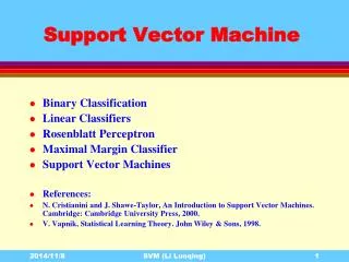
2. What is a Support Vector Machine? • An optimally defined surface • Linear or nonlinear in the input space • Linear in a higher dimensional feature space • Implicitly defined by a kernel function • K(A,B)  C

3. What are Support Vector Machines Used For? • Classification • Regression & Data Fitting • Supervised & Unsupervised Learning

4. Principal Topics • Knowledge-based classification • Incorporate expert knowledge into a classifier • Breast cancer prognosis & chemotherapy • Classify patients on basis of distinct survival curves • Isolate a class of patients that may benefit from chemotherapy • Multiple Myeloma detection via gene expression measurements • Drug discovery based on gene macroarray expression • Joint work with ExonHit

5. Support Vector MachinesMaximize the Margin between Bounding Planes A+ A-

6. Principal Topics • Knowledge-based classification (NIPS*2002)

7. Conventional Data-Based SVM

8. Knowledge-Based SVM via Polyhedral Knowledge Sets

9. Suppose that the knowledge set: belongs to the class A+. Hence it must lie in the halfspace : • We therefore have the implication: Incoporating Knowledge Sets Into an SVM Classifier • This implication is equivalent to a set of constraints that can be imposed on the classification problem.

10. Numerical TestingThe Promoter Recognition Dataset • Promoter: Short DNA sequence that precedes a gene sequence. • A promoter consists of 57 consecutive DNA nucleotides belonging to {A,G,C,T} . • Important to distinguish between promoters and nonpromoters • This distinction identifies starting locations of genes in long uncharacterizedDNA sequences.

11. The Promoter Recognition DatasetNumerical Representation • Simple “1 of N” mapping scheme for converting nominal attributes into a real valued representation: • Not most economical representation, but commonly used.

12. The Promoter Recognition DatasetNumerical Representation • Feature space mapped from 57-dimensional nominal space to a real valued 57 x 4=228 dimensional space. 57 nominal values 57 x 4 =228 binary values

13. Promoter Recognition Dataset Prior Knowledge Rules • Prior knowledge consist of the following 64 rules:

14. where denotes position of a nucleotide, with respect to a meaningful reference point starting at position and ending at position Then: Promoter Recognition Dataset Sample Rules

15. The Promoter Recognition DatasetComparative Algorithms • KBANN Knowledge-based artificial neural network [Shavlik et al] • BP: Standard back propagation for neural networks [Rumelhart et al] • O’Neill’s Method Empirical method suggested by biologist O’Neill [O’Neill] • NN: Nearest neighbor with k=3 [Cost et al] • ID3: Quinlan’s decision tree builder[Quinlan] • SVM1: Standard 1-norm SVM [Bradley et al]

16. The Promoter Recognition DatasetComparative Test Results

17. Principal Topics • Breast cancer prognosis & chemotherapy

18. Kaplan-Meier Curves for Overall Patients:With & Without Chemotherapy

19. Poor1: Lymph>=5 OR Tumor>=4 Compute Median Using 6 Features Good1: Lymph=0 AND Tumor<2 Compute Median Using 6 Features Compute Initial Cluster Centers Cluster 113 NoChemo Patients Use k-Median Algorithm with Initial Centers: Medians of Good1 & Poor1 Cluster 140 Chemo Patients Use k-Median Algorithm with Initial Centers: Medians of Good1 & Poor1 44 NoChemo Poor 67 Chemo Good 73 Chemo Poor 69 NoChemo Good Poor Intermediate Good Breast Cancer Prognosis & ChemotherapyGood, Intermediate & Poor Patient Groupings(6 Input Features : 5 Cytological, 1 Histological)(Clustering: Utilizes 2 Histological Features &Chemotherapy) 253 Patients (113 NoChemo, 140 Chemo)

20. Kaplan-Meier Survival Curvesfor Good, Intermediate & Poor Patients82.7% Classifier Correctness via 3 SVMs

21. Kaplan-Meier Survival Curves for Intermediate Group Note Reversed Role of Chemotherapy

22. Multiple Myeloma Detection • Multiple Myeloma is cancer of the plasma cell • Plasma cells normally produce antibodies • Out of control plasma cells produce tumors • When tumors appear in multiple sites they are called Multiple Myeloma • Dataset • 105 patients: 74 with MM, 31 healthy • Each patient is represented by 7008 gene measurements taken from plasma cell samples • For each one of the 7008 gene measurements • Absolute Call (AC): • Absent (A), Marginal (M) or Present (P) • Average Difference (AD): • Positive or negative number

23. Multiple Myeloma Data Representation A  1 0 0 M  0 1 0 P  0 0 1 AMP  7008 X 3 = 21024 AD  7008 Total = 28,032 per patient 104 Patients: 74 MM + 31 Healthy 104 X 28,032 Data Matrix A

24. Multiple Myeloma 1-Norm SVM Linear Classifier • Leave-one-out-correctness (looc) = 100% • Average number of features used = 7 per fold • Total computing time for 105 folds = 7892 sec. • Overall number of features used in 105 folds= 7

25. Breast Cancer Treatment ResponseJoint with ExonHit - Paris (Curie Dataset) • 35 patients treated by a drug cocktail • 9 partial responders; 26 nonresponders • 25 gene expressions out of 692, selected by Arnaud Zeboulon • Most patients had 3 replicate measurements • 1-Norm SVM classifier selected 14 out of 25 gene expressions • Leave-one-out correctness was 80% • Greedy combinatorial approach selected 5 genes out of 14 • Separating plane obtained in 5-dimensional gene-expression space • Replicates of all patients except one used in training • Average of replicates of patient left out used for testing • Leave-one-out correctness was 33 out of 35, or 94.2%

26. Separation of Convex Hull of Replicates of:10 Synthetic Nonresponders &4 Synthetic Partial Responders

27. Linear Classifier in 3-Gene Space35 Patients with 93 Replicates26 Nonresponders & 9 Partial Responders

28. Conclusion • New approaches for SVM-based classification • Algorithms capable of classifying data with few examples in very large dimensional spaces • Typical of microarray classification problems • Classifiers based on both abstract prior knowledge as well as conventional datasets • Identification of breast cancer patients that can benefit fromchemotherapy • Useful tool for drug discovery