Download
1 / 28
360 likes | 756 Views
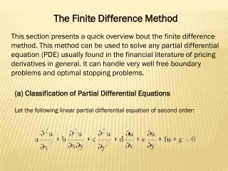
Finite Difference Method. For conductor exterior, solve Laplacian equation In 2D:. k. m. l. i. j. Uniform Grid. i, j+1. i+1, j. i – 1, j. i, j. i, j – 1. Basic Properties. Consider two conductors Let v=f(Q). From Gauss’ law

E N D
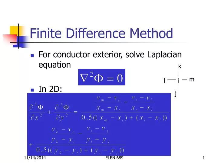
Finite Difference Method • For conductor exterior, solve Laplacian equation • In 2D: k m l i j ELEN 689
Uniform Grid i, j+1 i+1, j i–1, j i, j i, j–1 ELEN 689
Basic Properties • Consider two conductors • Let v=f(Q). From Gauss’ law if we double the amount of charge, E will also double since the equation is linear • Therefore, v and Q are linearly related, or Q=Cv +Q –Q S Really? ELEN 689
Multiple Conductors • Consider conductors 1, 2, …, n • Apply the above argument for every pair of conductors i and j Q1 Qn Q2 ELEN 689
Capacitance Matrix ELEN 689
BEM Review • Partition conductor surfaces into panels • Build coefficient matrix P, where and G is Green’s function, such as • Solve linear system Pq=v • Add charges to get capacitance ELEN 689
Make It Faster • Discretization: O(n) • Compute P: O(n2) O(n) • Since P is size nn, P can not be constructed explicitly • Solve Pq=v: O(n3) O(n) • Iterative methods ELEN 689
Fast Multipole Methods • N-body problem: Given n particles in 3D space, compute all forces between the particles • Fast multipole algorithms • Appel 85 • Rokhlin 86, Greengard & Rokhlin 87 • O(n) time ELEN 689
Basic Idea of Multipole • A cluster of charges at distance can be approximated by a single charge • Reduce operations from k2 to k • Form all clusters recursively in O(n) time — hard part! potential at k points k charges ELEN 689
Solve Ax=b Iteratively • Approximate Ax–b=0: • Bottleneck: Matrix-vector product Ax • A is not used elsewhere Initial solution x Compute Ax If Ax–b > t/b, modify x ELEN 689
Example: Jacobi Method ELEN 689
Example: Jacobi Method • Transformation • Ax = b Dx=Dx–Ax+b x = (I–D–1A)x+D–1b • Iterations • x(i+1)= (I–D–1A) x(i)+D–1b • x(0) = 0, x(1) = D–1b, x(2) = (I–D–1A) x(1)+D–1b, … • If diagonal dominate, then the method converges • Better iterative methods exist that converge under weaker conditions ELEN 689
Fast Algorithm HiCap • Conductor surface refinement: • Adaptively partition conductor surfaces into small panels according to a user supplied threshold • Approximate P and store it in a hierarchical data structure of size O(n) • The data structure permits O(n) time matrix-vector product Px for any n-vector x • Solve linear system Pq=v using iterative methods ELEN 689
5 1 2 3 4 Adaptive Panel Partition • If interaction between Ai Aj > , refine Ai and Aj. Otherwise, record Pij in P. C C A E B F G M N L I H J J ELEN 689
Representation of Matrix P • P is stored as links in a hierarchical data structure A H B C I J D E K L N G M F ELEN 689
Example • If area/dist 1, refine the panel A H 2 1/7 1/5 1/5 C B C I J 4 1/3 B 1 I 4 J ELEN 689
Example (cont’d) • If area/dist 1, refine the panel A H 2 1/7 1/5 1/5 C B C I J 4 E F G 1 D E K L M N L 4 N G M F J ELEN 689
A H Full 8x8 matrix P: B I J C K E D L D B E A C 1/4.6 M K N 1/4.6 I 1/5.5 L H J
A H Implicitly stored P: B I J C K E D L D B E A C 1/5 K I L H J
Properties of P • P positive, symmetric, positive definite • Positive definite: xPx > 0 for all x • If fully expanded, P is size nn • P can be approximated by O(n) block entries, where n is the number of panels • This is because each panel interacts with constant number of other panels • The block entries allow O(n) time matrix-vector product Px for any x ELEN 689
Mat-Vec Pq, Step 1 • Compute charge for all panels A H B C I J D E K L N G M F ELEN 689
Mat-Vec Pq, Step 2 • Compute potential for all panels A H B C I J D E K L N G M F ELEN 689
Mat-Vec Pq, Step 3 • Distribute potential to leaf panels A H B C I J D E K L N G M F ELEN 689
Solving Linear Systems • Use fast iterative methods GMRES • Each iteration requires a matrix-vector product Pq that can be completed in O(n) time • Solution obtained in 10-20 iterations, regardless of n ELEN 689
Error and Time Complexity • Error of approximation is controlled by • Time complexity is O(n) because step takes O(n) time ELEN 689
Multi-layer Dielectric • Kernel independent methods • Multi-layer Green’s function • Kernel dependent methods • Discretize dielectric-dielectric interface • Introduce interface variables and modify linear system • Expensive =8.0 m3 =4.0 m2 m2 m2 =3.9 =4.1 m1 ELEN 689
Other Dielectric Problems • Conformal dielectric • Voids • Air gap m3 m2 m2 m1 ELEN 689
Comparison of Methods • FastCap: O(n) • Kernel dependent (1/r) • Random Walk • Kernel independent, QuickCap • Pre-corrected FFT: O(nlogn) • Kernel independent • Singular Value Decomposition: O(nlogn) • Kernel independent, Assura RCX • HiCap: O(n) • Kernel independent ELEN 689