Download
1 / 15
150 likes | 152 Views
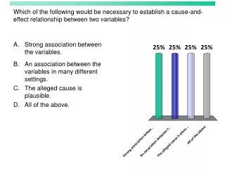
Association between Variables Measured at the Nominal Level. Introduction. The measures of association are more efficient methods of expressing an association than calculating percentages for bivariate tables—they express the relationship in a single number

E N D
Introduction • The measures of association are more efficient methods of expressing an association than calculating percentages for bivariate tables—they express the relationship in a single number • However, we always need to look at the percentages in the bivariate tables (crosstabs), since a single number loses some information
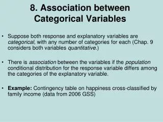
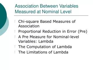
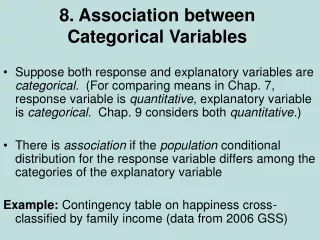
Many Different Measures of Association • Different ones are used for different levels of measurement (nominal, ordinal, or interval/ratio) • When selecting measures of association for variables measured at different levels, social scientists generally choose the measure that is appropriate for the lower of the levels • So if one variable is nominal, and the other interval, you would use a level of association appropriate for the nominal variable
Chi-Square-Based Measures of Association • These have been commonly used, since we already have calculated chi square for inferential statistics; it is simple to transform it into a measure of association • We can see from the percentages in a bivariate table that two variables are associated, and know from chi square that the differences are statistically significant
Interpretation of Cramer’s V • It has an upper limit of 1.00 for any size table • It is interpreted as an index that measures the strength of the association between two variables • A major problem with Cramer’s V is the absence of a direct or meaningful interpretation for values between the extremes of 0.00 and 1.00
Proportional Reduction in Error (PRE) • For nominal-level variables, the logic of PRE involves first attempting to guess or predict the category into which each case will fall on the dependent variable (Y) while ignoring the independent variable (X) • Will be predicting blindly in this case, and will make many errors • The second step would be to predict again the category of each case on the dependent variable, but take the independent variable into account
PRE, cont. • If the two variables are associated, the additional information from the independent variable should enable us to reduce our errors of prediction • The stronger the association between the variables, the more we will reduce our errors • In the case of a perfect association, we would make no errors at all when predicting scores on Y from scores on X • When there is no association between the variables, knowledge of the independent will not improve the accuracy of our predictions—we would make just as many errors of prediction
Lambda • Lambda is a PRE measure for nominal-level variables • We know that gender and height are associated by looking at the percentages • To measure the strength of this association, a PRE measure called lambda will be calculated • First need to find the number of prediction errors made while ignoring the independent variable (gender) • Then will find the number of prediction errors made while taking gender into account • These two sums will be compared
Example of Height by Gender • We can predict either that all subjects are tall or that all subjects are short (these are the only two permitted by lambda) • Clearly, gender and height are associated, since we made fewer errors of prediction while considering gender than while ignoring gender
Interpretation of Lambda • For the above example, lambda equals .71 • Lambda has a possible range of 0 to 1 • A lambda of 0 would indicate that the information given by the independent variable does not improve our ability to predict the dependent and therefore, that there is no association between the variables • A lambda of 1.00 would mean that it was possible to predict Y without error from X
PRE Interpretation • Additionally, lambda allows a direct and meaningful interpretation of the numbers in between • When multiplied by 100, the value of lambda indicates directly the proportional reduction in error—the strength of the association • So, a lambda of .71 tells us that knowledge of gender improves our ability to predict height by a factor of 71% • Of, we are 71% better off knowing gender when attempting to predict height than we are not knowing gender
Other Examples • If lambda = .20, this indicates that we are 20% better off knowing the independent variable when attempting to predict a person’s score or value on the dependent variable • If we make 75 errors when predicting Y without knowledge of X, and 60 errors when predicting Y with knowledge of X, then X and Y are associated • If the value of lambda is relatively low, we may conclude that other variables are importantly associated with the dependent variable
Problems with Lambda • It changes if you reverse the independent and dependent variables • Need to follow the convention of putting the independent variable in the columns and compute lambda as done above • You also need to be confident which variable is the independent one and which is the dependent one
Second Problem • If one of the row totals is much larger than the others, lambda can take on a value of 0 even when other measures of association would not be 0, and calculating percentages for the table indicates some association between the variables • Suggests that you use great caution in interpretation of lambda when the row marginals are very unequal • If the row totals are unequal, you should use a chi-square-based measure of association (phi or Cramer’s V) • For the same bivariate table, Cramer’s V is .27 and lambda is zero, we can conclude that the variables may be associated even if lambda is zero—need to disregard lambda if the row marginals are very unequal