Download
1 / 40
400 likes | 404 Views
This article discusses microarray analysis for differentiating two biological conditions, such as Acute Lymphocytic Leukemia (ALL) and Acute Myelogenous Leukemia (AML), based on gene expression patterns. It explores the geometric formulation, hyperplane separation, and various classification methods such as Rosenblatt's perceptron learning algorithm and Linear Discriminant Analysis (LDA).

E N D
The Biological Problem • Two conditions that need to be differentiated, (Have different treatments). • EX: ALL (Acute Lymphocytic Leukemia) & AML (Acute Myelogenous Leukima) • Possibly, the set of genes over-expressed are different in the two conditions
Geometric formulation • Each sample is a vector with dimension equal to the number of genes. • We have two classes of vectors (AML, ALL), and would like to separate them, if possible, with a hyperplane.
Basic geometry • What is ||x||2 ? • What is x/||x|| • Dot product? x=(x1,x2) y
Dot Product x • Let be a unit vector. • |||| = 1 • Recall that • Tx = ||x|| cos • What is Tx if x is orthogonal (perpendicular) to ? Tx = ||x|| cos
Find the unit vector that is perpendicular (normal to the hyperplane) Hyperplane • How can we define a hyperplane L?
Points on the hyperplane • Consider a hyperplane L defined by unit vector , and distance 0 from the origin • Notes; • For all x L, xTmust be the same, xT = 0 • For any two points x1, x2, • (x1- x2)T =0 • Therefore, given a vector , and an offset 0, the hyperplane is the set of all points • {x : xT = 0} x2 x1
Hyperplane properties • Given an arbitrary point x, what is the distance from x to the plane L? • D(x,L) = (Tx -0) • When are points x1 and x2 on different sides of the hyperplane? x 0
Hyperplane properties • Given an arbitrary point x, what is the distance from x to the plane L? • D(x,L) = (Tx -0) • When are points x1 and x2 on different sides of the hyperplane? • Ans: If D(x1,L)* D(x2,L) < 0 x 0
+ x2 - x1 Separating by a hyperplane • Input: A training set of +ve & -ve examples • Recall that a hyperplane is represented by • {x:-0+1x1+2x2=0} or • (in higher dimensions) {x: Tx-0=0} • Goal: Find a hyperplane that ‘separates’ the two classes. • Classification: A new point x is +ve if it lies on the +ve side of the hyperplane (D(x,L)> 0) , -ve otherwise.
Hyperplane separation • What happens if we have many choices of a hyperplane? • We try to maximize the distance of the points from the hyperplane. • What happens if the classes are not separable by a hyperplane? • We define a function based on the amount of mis-classification, and try to minimize it
Error in classification • Sample Function: sum of distances of all misclassified points • Let yi=-1 for +ve example i, yi=+1 otherwise. • The best hyperplane is one that minimizes D(,0) • Other definitions are also possible. + x2 - x1
Restating Classification • The (supervised) classification problem can now be reformulated as an optimization problem. • Goal: Find the hyperplane (,0), that optimizes the objective D(,0). • No efficient algorithm is known for this problem, but a simple generic optimization can be applied. • Start with a randomly chosen (,0) • Move to a neighboring (’,’0) if D(’,’0)< D(,0)
Gradient Descent • The function D() defines the error. • We follow an iterative refinement. In each step, refine so the error is reduced. • Gradient descent is an approach to such iterative refinement. D() D’()
Classification based on perceptron learning • Use Rosenblatt’s algorithm to compute the hyperplane L=(,0). • Assign x to class 1 if D(x,L)= Tx-0 >= 0, and to class 2 otherwise. x 0
Perceptron learning • If many solutions are possible, it does no choose between solutions • If data is not linearly separable, it does not terminate, and it is hard to detect. • Time of convergence is not well understood
+ x2 - x1 Linear Discriminant analysis • Provides an alternative approach to classification with a linear function. • Project all points, including the means, onto vector . • We want to choose such that • Difference of projected means is large. • Variance within group is small
+ + 1 x2 x2 - - 2 x1 x1 Choosing the right • 1 is a better choice than 2 as the variance within a group is small, and difference of means is large. • How do we compute the best ?
Linear Discriminant analysis • Fisher Criterion
+ x2 - x1 LDA cont’d • What is the projection of a point x onto ? • Ans: Tx • What is the distance between projected means? x
LDA Cont’d Fisher Criterion
LDA Therefore, a simple computation (Matrix inverse) is sufficient to compute the ‘best’ separating hyperplane
Maximum Likelihood discrimination • Consider the simple case of single dimensional data. • Compute a distribution of the values in each class. values Pr
Maximum Likelihood discrimination • Suppose we knew the distribution of points in each class i. • We can compute Pr(x|i) for all classes i, and take the maximum • The true distribution is not known, so usually, we assume that it is Gaussian
ML discrimination • Suppose all the points were in 1 dimension, and all classes were normally distributed. 1 x 2
ML discrimination (multi-dimensional case) Not part of the syllabus.
Supervised classification summary • Most techniques for supervised classification are based on the notion of a separating hyperplane. • The ‘optimal’ separation can be computed using various combinatorial (perceptron), algebraic (LDA), or statistical (ML) analyses.
Dimensionality reduction • Many genes have highly correlated expression profiles. • By discarding some of the genes, we can greatly reduce the dimensionality of the problem. • There are other, more principled ways to do such dimensionality reduction.
Principle Components Analysis • Consider the expression values of 2 genes over 6 samples. • Clearly, the expression of the two genes is highly correlated. • Projecting all the genes on a single line could explain most of the data. • This is a generalization of “discarding the gene”.
PCA • Suppose all of the data were to be reduced by projecting to a single line from the mean. • How do we select the line ? m
PCA cont’d • Let each point xk map to x’k. We want to mimimize the error • Observation 1: Each point xk maps to x’k = m + T(xk-m) xk x’k m
PCA: motivating example • Consider the expression values of 2 genes over 6 samples. • Clearly, the expression of g1 is not informative, and it suffices to look at g2 values. • Dimensionality can be reduced by discarding the gene g1 g1 g2
PCA: Ex2 • Consider the expression values of 2 genes over 6 samples. • Clearly, the expression of the two genes is highly correlated. • Projecting all the genes on a single line could explain most of the data.
PCA • Suppose all of the data were to be reduced by projecting to a single line from the mean. • How do we select the line ? m
PCA cont’d • Let each point xk map to x’k=m+ak. We want to minimize the error • Observation 1: Each point xk maps to x’k = m + T(xk-m) • (ak= T(xk-m)) xk x’k m
Proof of Observation 1 Differentiating w.r.t ak
Minimizing PCA Error • To minimize error, we must maximize TS • By definition, = TS implies that is an eigenvalue, and the corresponding eigenvector. • Therefore, we must choose the eigenvector corresponding to the largest eigenvalue.
PCA • The single best dimension is given by the eigenvector of the largest eigenvalue of S • The best k dimensions can be obtained by the eigenvectors {1, 2, …, k} corresponding to the k largest eigenvalues. • To obtain the k dimensional surface, take BTM 1T BT M