Component Analysis Techniques for Dimension Reduction and Classification

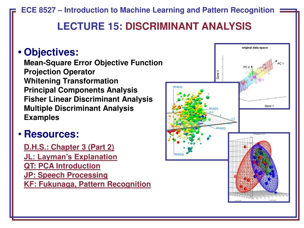
1. LECTURE 15: DISCRIMINANT ANALYSIS • • Objectives:Mean-Square Error Objective FunctionProjection OperatorWhitening TransformationPrincipal Components AnalysisFisher Linear Discriminant AnalysisMultiple Discriminant AnalysisExamples • Resources: • D.H.S.: Chapter 3 (Part 2)JL: Layman’s ExplanationQT: PCA IntroductionJP: Speech ProcessingKF: Fukunaga, Pattern Recognition

2. Component Analysis • Component analysis is a technique that combines features to reduce the dimension of the feature space. • It can also be the basis for a classification algorithm. • Features of this approach include: • Statistical decorrelation of the data. • Linear combinations are simple to compute and tractable. • Project a high dimensional space onto a lower dimensional space. • Gain insight into the relative importance of each feature. • Three classical approaches for finding the optimal transformation: • Principal Components Analysis (PCA): projection that best represents the data in a least-square sense. • Multiple Discriminant Analysis (MDA): projection that best separates the data in a least-squares sense. • Independent Component Analysis (IDA): projection that minimizes the mutual information of the components.

3. Principal Component Analysis • Consider representing a set of n d-dimensional samples x1,…,xnby a single vector, x0. • Define a squared-error criterion: • The solution to this problem is given by: • The sample mean is a zero-dimensional representation of the data set. • Consider a one-dimensional solution: • In other words, the best one-dimensional projection of the data (in the least mean-squared error sense) is the projection of the data onto a line through the sample mean in the direction of the eigenvector of the scatter matrix having the largest eigenvalue (hence the name Principal Component). • For the Gaussian case, the eigenvectors are the principal axes of the hyperellipsoidally shaped support region!

4. Alternate View: Coordinate Transformations • Why is it convenient to convert an arbitrary distribution into a spherical one? (Hint: Euclidean distance) • Consider the transformation: Aw= ΦΛ-1/2 • where Φ is the matrix whose columns are the orthonormal eigenvectors of Σ and Λ is a diagonal matrix of eigenvalues (Σ= ΦΛΦt). Note that Φ is unitary. • What is the covariance of y=Awx? • E[yyt] = (Awx)(Awx)t =(Φ Λ-1/2x)(Φ Λ-1/2x)t • = Φ Λ-1/2xxt Λ-1/2 Φt = ΦΛ-1/2 ΣΛ-1/2 Φt • = ΦΛ-1/2 ΦΛΦtΛ-1/2 Φt • = (ΦΦt) (Λ-1/2 ΛΛ-1/2 )(ΦΦt) • = I • Why is this significant?

5. Examples of Maximum Likelihood Classification • For the Gaussian case, the eigenvectors are the principal axes of the hyperellipsoidally shaped support region! • Let’s work some examples (class-independent and class-dependent PCA). • In class-independent PCA, a global covariance matrix is computed: • In this case, the covariance will be an ellipsoid. • The first principal component will be the major axis of this ellipsoid. • The second principal component will be the minor axis. • In class-dependent PCA, which requires labeled training data, transformations are computed independently for each class. • The ML decision surface is a line (or a parabola in this case).

6. Discriminant Analysis • Discriminant analysis seeks directions that are efficient for discrimination. • Consider the problem of projecting data from d dimensions onto a line with the hope that we can optimize the orientation of the line to minimize error. • Consider a set of n d-dimensional samples x1,…,xnin the subset D1 labeled 1 and n2 in the subset D2 labeled 2. • Define a linear combination of x: • and a corresponding set of n samples y1, …, yndivided into Y1 and Y2. • Our challenge is to find w that maximizes separation. • This can be done by considering the ratio of the between-class scatter to the within-class scatter.

7. Separation of the Means and Scatter • Define a sample mean for class i: • The sample mean for the projected points are: • The sample mean for the projected points is just the projection of the mean (which is expected since this is a linear transformation). • It follows that the distance between the projected means is: • Define a scatter for the projected samples: • An estimate of the variance of the pooled data is: • and is called the within-class scatter.

8. Fisher Linear Discriminant and Scatter • The Fisher linear discriminant maximizes the criteria: • Define a scatter for class I, Si : • The total scatter, Sw, is: • We can write the scatter for the projected samples as: • Therefore, the sum of the scatters can be written as:

9. Separation of the Projected Means • The separation of the projected means obeys: • Where the between class scatter, SB, is given by: • Sw is the within-class scatter and is proportional to the covariance of the pooled data. • SB , the between-class scatter, is symmetric and positive definite, but because it is the outer product of two vectors, its rank is at most one. • This implies that for any w, SBw is in the direction of m1-m2. • The criterion function, J(w), can be written as:

10. Linear Discriminant Analysis • This ratio is well-known as the generalized Rayleigh quotient and has the well-known property that the vector, w, that maximizes J(), must satisfy: • The solution is: • This is Fisher’s linear discriminant, also known as the canonical variate. • This solution maps the d-dimensional problem to a one-dimensional problem (in this case). • From Chapter 2, when the conditional densities, p(x|i), are multivariate normal with equal covariances, the optimal decision boundary is given by: • where , and w0 is related to the prior probabilities. • The computational complexity is dominated by the calculation of the within-class scatter and its inverse, an O(d2n) calculation. But this is done offline! • Let’s work some examples (class-independent PCA and LDA).

11. Multiple Discriminant Analysis • For the c-class problem in a d-dimensional space, the natural generalization involves c-1 discriminant functions. • The within-class scatter is defined as: • Define a total mean vector, m: • and a total scatter matrix, ST, by: • The total scatter is related to the within-class scatter (derivation omitted): • We have c-1 discriminant functions of the form:

12. Multiple Discriminant Analysis (Cont.) • The criterion function is: • The solution to maximizing J(W) is once again found via an eigenvalue decomposition: • Because SB is the sum of c rank one or less matrices, and because only c-1 of these are independent, SB is of rank c-1 or less. • An excellent presentation on applications of LDA can be found at PCA Fails!

13. Summary • Principal Component Analysis (PCA): represents the data by minimizing the squared error (representing data in directions of greatest variance). • PCA is commonly applied in a class-dependent manner where a whitening transformation is computed for each class, and the distance from the mean of that class is measured using this class-specific transformation. • PCA gives insight into the important dimensions of your problem by examining the direction of the eigenvectors. • Linear DIscriminant Analysis (LDA): attempts to project the data onto a line that represents the direction of maximum discrimination. • LDA can be generalized to a multi-class problem through the use of multiple discriminant functions (c classes require c-1 discriminant functions).