Download
1 / 20
330 likes | 850 Views
Real-time Optimization. Introduction Motivating example Unconstrained optimization Constrained optimization Matlab example. Introduction. Optimization problems are ubiquitous in chemical engineering Process and equipment design Model parameter estimation Data reconciliation

E N D
Real-time Optimization • Introduction • Motivating example • Unconstrained optimization • Constrained optimization • Matlab example
Introduction • Optimization problems are ubiquitous in chemical engineering • Process and equipment design • Model parameter estimation • Data reconciliation • Optimal steady-state operation • Optimal dynamic control • Scheduling and planning • Our focus • Real-time optimization • Problem formulation and characteristics • Available software tools
Regulatory control Maintain outputs at specified setpoints No optimization Multivariable control Drive process to desired steady-state operating point Control moves determined via dynamic optimization Covered in next lecture Real-time optimization Determine most favorable steady-state operating point Steady-state determined via optimization Real-Time Optimization (RTO)
RTO System Implementation • Control – maintain process at setpoints • Data reconciliation – adjust measurements to satisfy material and energy balances • Parameter estimation – adjust model parameters to match model to process data • Steady-state optimization – determine steady-state operating point that maximizes profit
Formulation of RTO Problems • Basic requirements • Economic model – an objective function to be maximized or minimized • Operating model – a steady-state process model and constraints on the process variables • Basic procedure • Identify the input and output variables • Select the objective function • Develop the process model and constraints • Simplify the objective function and process model if necessary • Compute the optimal solution • Perform sensitivity analysis
Motivating Example • Optimization problem • Determine the steady-state production rates of E and F that maximize operating profit • Reactions • Process 1: A+B E • Process 2: A+2B F
Problem Formulation • Variables • x1 = lb/day A consumed • x2= lb/day B consumed • x3 = lb/day E produced • x4 = lb/day F produced • Operating profit ($/day): • Sales income = 0.4x3+0.33x4 • Feed cost = 0.15x1+0.2x2 • Operating cost = 0.15x3+0.05x4+350+200 • Total profit: P = 0.25x3+0.28x4-0.15x1-0.2x2-550
Problem Formulation cont. • Material balances constraints • x1 = 0.667x3+0.5x4 • x2 = 0.333x3+0.5x4 • Variable constraints • 0 < x1 < 40,000 • 0 < x2 < 30,000 • 0 < x3 < 30,000 • 0 < x4 < 30,000 • Optimization problem • Determine x1, x2, x3 and x4 that maximize P while satisfying material balance and variable constraints • Example of a linear program • Matlab solution: x1 = 35010, x2 = 24990, x3 = 30000, x4 = 30000, P = 5651
Single Variable Optimization • Examples • Optimal reflux rate in a distillation column • Optimal air/fuel ratio in a furnace • Unconstrained problem: • Easily solved in Excel, Matlab, Mathcad, etc. • Conceptual solution • Assume function is unimodal with only one extremum • Newton’s method • Convergence may require good initial guess
Multivariable Optimization • Examples • Optimal reflux rate and boilup rate in a distillation column • Optimal air/fuel ratio and temperature in a furnace • Unconstrained problem: • Conceptual solution • Requires more sophisticated algorithms and software tools • Optimization toolbox in Matlab
Constrained Optimization • General constrained optimization problem • Constraints • Active constraints – limit optimal solution • Inactive constraints – do not limit optimal solution • Optimal solution often located at intersection of active constraints
Linear Programming • Characteristics • Linear objective function • Linear equality and inequality constraints • Examples of linear constraints • Production and raw material limitations • Product specifications • Safety requirements • Material and energy balances • Linear program (LP)
Solution of Linear Programs • Key property • Optimal solution lies on domain boundary at the intersection of active constraints (vertices) • Only a finite number of vertices must be checked • Allows huge reduction in computation cost • Simplex algorithm • Most widely used LP solution method • Provides efficient of very large LPs
Quadratic Programming • Characteristics • Quadratic objective function • Linear equality and inequality constraints • Examples of quadratic objective functions • Least-squares parameter estimation problems • Multivariable control problems (next lecture) • Quadratic program (QP) • Very efficient solution methods available
Convexity • Convex function • A function is convex if the function lies below a line connecting any two points in the domain • Convex set • A set is convex if a line connecting any two points in the set is completely contained within the set • The intersection of convex sets yields a convex set • Convex optimization problem • A convex objective function and convex constraints yields a convex optimization problem • Possesses a single global optima • Linear and quadratic programming problems are convex
f(x) x Nonlinear Programming • Nonlinear program (NLP) • Generally not convex • Often exhibit multiple optima • Goal is to determine the global optima • Solution methods • Many NLP solution codes are available • “Best” code is highly problem dependent • Most codes provide no guarantee of global optimality • Usuallt necessary to rerun code with multiple initial guesses
NLP Solution • Successive quadratic programming (SQP) methods • Approximate NLP as sequence of QPs • Require first-order derivatives (Jacobian matrix) and second-order derivatives (Hessian matrix) • Codes: NPSOL, SNOPT • Generalized-reduced gradient (GRG) methods • Solve sequence of simplified NLPs • Require first-order and second-order derivatives • Codes: Excel, GRG2, CONOPT • Derivative-free methods • Direct search, genetic and simulated annealing algorithms • Allow determination of global optima but very slow • Practical issues • “Best” code is highly problem dependent • Most codes provide no guarantee of global optimality • Usually necessary to rerun code with multiple initial guesses • The Matlab optimization toolbox provides numerous functions to solve LP, QP and NLP problems
Exit Gas Flow Fresh Media Feed (substrates) Agitator Exit Liquid Flow (cells & products) Matlab Example
Optimization Problem Formulation • Objective function • Maximize steady-state productivity: Q = DP • Decision variables • Dilution rate and feed substrate concentration (D, Sf) • Biomass, substrate and product concentrations (X, S, P) • Equality constraints • Nonlinear program • Matlab solution: X = 7.30, S = 5.14, P = 25.00, D = 0.164, Sf= 23.4, Q = 4.09