Download
1 / 34
350 likes | 476 Views
Memory Hierarchies & Optimizations Case Study: Tuning Matrix Multiply. Based on slides by: Kathy Yelick www.cs.berkeley.edu/~yelick/cs194f07 & James Demmel and Horst Simon http://www.cs.berkeley.edu/~demmel/cs267_Spr10/. Motivation.

E N D
Memory Hierarchies & Optimizations Case Study: Tuning Matrix Multiply Based on slides by: Kathy Yelick www.cs.berkeley.edu/~yelick/cs194f07 & James Demmel and Horst Simon http://www.cs.berkeley.edu/~demmel/cs267_Spr10/ CPE 779 Parallel Computing - Spring 2010
Motivation • Most applications run at < 10% of the “peak” performance of a system • Peak is the maximum the hardware can physically execute • Much of this performance is lost on a single processor, i.e., the code running on one processor often runs at only 10-20% of the processor peak • Most of the single processor performance loss is in the memory system • Moving data takes much longer than arithmetic and logic • A parallel programmer is also a performanceprogrammer • Understand your hardware • To understand this, we need to look under the hood of modern processors • In these slides, we will look at only a single “core” processor • These issues will exist on processors within any parallel computer
Outline • Idealized and actual costs in modern processors • Parallelism within single processors • Memory hierarchies • Use of microbenchmarks to characterized performance • Case study: Matrix Multiplication • Use of performance models to understand performance CPE 779 Parallel Computing - Spring 2010
Outline • Idealized and actual costs in modern processors • Parallelism within single processors • Memory hierarchies • Use of microbenchmarks to characterized performance • Case study: Matrix Multiplication • Use of performance models to understand performance CPE 779 Parallel Computing - Spring 2010
Idealized Uniprocessor Model • Processor names bytes, words, etc. in its address space • These represent integers, floats, pointers, arrays, etc. • Operations include • Read and write into very fast memory called registers • Arithmetic and other logical operations on registers • Order specified by program • Read returns the most recently written data • Compiler and architecture translate high level expressions into “obvious” lower level instructions • Hardware executes instructions in order specified by compiler • Idealized Cost • Each operation has roughly the same cost (read, write, add, multiply, etc.) Read address(B) to R1 Read address(C) to R2 R3 = R1 + R2 Write R3 to Address(A) A = B + C CPE 779 Parallel Computing - Spring 2010
Uniprocessors in the Real World • Real processors have • registers and caches • small amounts of fast memory • store values of recently used or nearby data • different memory ops can have very different costs • parallelism • multiple “functional units” that can run in parallel • different instruction orders & instruction mixes have different costs • pipelining • a form of parallelism, like an assembly line in a factory • Why is this a problem for the programmer? • In theory, compilers understand all of this and can optimize your program; in practice they don’t. • Even if they could optimize one algorithm, they won’t know about a different algorithm that might be a much better “match” to the processor CPE 779 Parallel Computing - Spring 2010
Outline • Idealized and actual costs in modern processors • Parallelism within a processor • Hidden from software (sort of) • Pipelining • SIMD units • Memory hierarchies • Use of microbenchmarks to characterized performance • Case study: Matrix Multiplication • Use of performance models to understand performance CPE 779 Parallel Computing - Spring 2010
30 40 40 40 40 20 A B C D What is Pipelining? Dave Patterson’s Laundry example: 4 people doing laundry wash (30 min) + dry (40 min) + fold (20 min) = 90 min Latency • In this example: • Sequential execution takes 4 * 90min = 6 hours • Pipelined execution takes 30+4*40+20 = 3.5 hours • Bandwidth = loads/hour • BW = 4/6 l/h w/o pipelining • BW = 4/3.5= 1.14 l/h w pipelining • BW <= 1.5 l/h w pipelining, >>>>> more total loads • Pipelining helps bandwidth but not latency (90 min) • Bandwidth limited by slowest pipeline stage • Max speedup proportional to Number pipe stages 6 PM 7 8 9 Time T a s k O r d e r CPE 779 Parallel Computing - Spring 2010
MEM/WB ID/EX EX/MEM IF/ID Adder 4 Address ALU Example: 5 Steps of MIPS DatapathFigure 3.4, Page 134 , CA:AQA 2e by Patterson and Hennessy Instruction Fetch Execute Addr. Calc Memory Access Instr. Decode Reg. Fetch Write Back Next PC MUX Next SEQ PC Next SEQ PC Zero? RS1 Reg File MUX Memory RS2 Data Memory MUX MUX Sign Extend WB Data Imm RD RD RD • Pipelining is also used within arithmetic units • a fp multiply may have latency 10 cycles, but throughput of 1/cycle CPE 779 Parallel Computing - Spring 2010
SIMD: Single Instruction, Multiple Data • Scalar processing • traditional mode • one instruction producesone result • SIMD processing • one instruction produces multiple results • Accomplished in Intel processors with SSE (Streaming SIMD Extensions) & SSE2 instructions x3 x2 x1 x0 X X + + Y y3 y2 y1 y0 Y X + Y x3+y3 x2+y2 x1+y1 x0+y0 X + Y Slide Source: Alex Klimovitski & Dean Macri, Intel Corporation CPE 779 Parallel Computing - Spring 2010
SSE / SSE2 SIMD on Intel • SSE2 data types: anything that fits into a16 bytes register, e.g., • Instructions perform add, multiply etc. on all the data in a16-byte register in parallel • Challenges: • Need to be contiguous in memory • Some instructions to move data around from one part of register to another 4x floats 2x doubles 16x bytes CPE 779 Parallel Computing - Spring 2010
What does this mean to you (the programmer)? • In addition to SIMD extensions, the processor may have other special instructions • Fused Multiply-Add (FMA) instructions: x = y + c * z is so common that some processor execute the multiply/add as a single instruction, at the same rate (bandwidth) as + or * alone • In theory, the compiler understands all of this • When compiling, it will rearrange instructions to get a good “schedule” that maximizes pipelining, uses FMAs and SIMD • It works with the mix of instructions inside an inner loop or other block of code • But in practice the compiler may need your help • Choose a different compiler, optimization flags, etc. • Rearrange your code to make things more obvious • Using special functions (“intrinsics”) or write in assembly CPE 779 Parallel Computing - Spring 2010
Peak Performance • Whenever you look at performance, it’s useful to understand what you’re expecting • Machine peak is the maximum number of arithmetic operations a processor (or set of them) can perform • Often referred to as “speed of light” or “guaranteed not to exceed” number • Treat integer and floating point separately and be clear on how wide the operands are (# bits) • If you see a number higher than peak, you have a mistake in your timers, formulas, or … CPE 779 Parallel Computing - Spring 2010
Outline • Idealized and actual costs in modern processors • Parallelism within single processors • Memory hierarchies • Temporal and spatial locality • Basics of caches • Use of microbenchmarks to characterized performance • Case study: Matrix Multiplication • Use of performance models to understand performance CPE 779 Parallel Computing - Spring 2010
Memory Hierarchy • Most programs have a high degree of locality in their accesses • spatial locality: accessing things nearby previous accesses • temporal locality: reusing an item that was previously accessed • Memory hierarchy tries to exploit locality processor control Second level cache (SRAM) Secondary storage (Disk) Main memory (DRAM) Tertiary storage (Disk/Tape) datapath on-chip cache registers
: The Memory Wall Processor-DRAM Gap (latency) • Memory hierarchies are getting deeper • Processors get faster more quickly than memory µProc 60%/yr. 1000 CPU “Moore’s Law” 100 Processor-Memory Performance Gap:(grows 50% / year) Performance 10 DRAM 7%/yr. DRAM 1 1980 1981 1982 1983 1984 1985 1986 1987 1988 1989 1990 1991 1992 1993 1994 1995 1996 1997 1998 1999 2000 Time CPE 779 Parallel Computing - Spring 2010
Approaches to Handling Memory Latency • Bandwidth has improved more than latency • 23% per year vs 7% per year • Approach to address the memory latency problem • Eliminate memory operations by saving values in small, fast memory (cache) and reusing them • need temporal locality in program • Take advantage of better bandwidth by getting a chunk of data from memory and saving it in small fast memory (cache) and using whole chunk • need spatial locality in program • Take advantage of better bandwidth by allowing processor to issue multiple reads to the memory system at once • concurrency in the instruction stream, e.g. load whole array, as in vector processors; prefetching • Overlap computation & memory operations • prefetching CPE 779 Parallel Computing - Spring 2010
Cache Basics • Cache is fast (expensive) memory which keeps copy of data in main memory; it is hidden from software • Simplest example: data at memory address xxxxx1101 is stored at cache location 1101 • Cache hit: in-cache memory access—cheap • Cache miss: non-cached memory access—expensive • Need to access next, slower level of cache CPE 779 Parallel Computing - Spring 2010
Cache Basics (continued ) • Cache line length: # of bytes loaded together • Ex: If either xxxxx1100 or xxxxx1101 is accessed, both are loaded • Cache associativity • direct-mapped: 1 memory address is mapped to only 1 location in cache • A data line stored at address xxxxx1101 in memory is stored in cache location 1101, in a 16 locations cache • n-way associative: A data line stored at address xxxxx1101 can be stored in any of n cache locations (16 n 2 ; in a 16 locations cache ) • Up to n lines with addresses xxxxx1101 can be stored at cache location 1101 (so cache can store 16n lines) • Fully associative: 16-way associative (n=16) in a 16 locations cache CPE 779 Parallel Computing - Spring 2010
Why Have Multiple Levels of Cache? • On-chip vs. off-chip • On-chip caches are faster, but limited in size • A large cache has delays • Hardware to check longer addresses in cache takes more time • Associativity, which gives a more general set of data in cache, also takes more time • Example: • Cray T3E eliminated one cache to speed up misses • There are other levels of the memory hierarchy • Registers, pages (TLB, virtual memory), … • And it isn’t always a hierarchy CPE 779 Parallel Computing - Spring 2010
s • for array A of length L from 4KB to 8MB by 2x • for stride s from 4 Bytes (1 word) to L/2 by 2x • time the following loop • (repeat many times and average) • for i from 0 to L by s • load A[i] from memory (4 Bytes) Experimental Study of Memory (Membench) • Microbenchmark for memory system performance time the following loop (repeat many times and average) for i from 0 to L load A[i] from memory (4 Bytes) ments 1 experiment CPE 779 Parallel Computing - Spring 2010
memory time size > L1 cache hit time size < L1 Membench: What to Expect average cost per access • Consider the average cost per load • Plot one line for each array length; time vs. stride s • Small stride is best: if cache line holds 4 words, at most ¼ miss • If array is smaller than a given cache, all those accesses will hit (after the first run, which is negligible for large enough runs) • Picture assumes only one level of cache • Values have gotten more difficult to measure on modern procs s = stride CPE 779 Parallel Computing - Spring 2010
Mem: 396 ns (132 cycles) L2: 2 MB, 12 cycles (36 ns) L1: 16 KB 2 cycles (6ns) L1: 16 B line L2: 64 byte line 8 K pages, 32 TLB entries Memory Hierarchy on a Sun Ultra-2i Sun Ultra-2i, 333 MHz Array length See www.cs.berkeley.edu/~yelick/arvindk/t3d-isca95.ps for details CPE 779 Parallel Computing - Spring 2010
Lessons • Actual performance of a simple program can be a complicated function of the architecture • Slight changes in the architecture or program change the performance significantly • To write fast programs, need to consider architecture • True on sequential or parallel processor • We would like simple models to help us design efficient algorithms • We will illustrate with a common technique for improving cache performance, called blocking or tiling • Idea: use divide-and-conquer to define a problem that fits in register/L1-cache/L2-cache CPE 779 Parallel Computing - Spring 2010
Outline • Idealized and actual costs in modern processors • Parallelism within single processors • Memory hierarchies • Use of microbenchmarks to characterized performance • Case study: Matrix Multiplication • Use of performance models to understand performance • Simple cache model • Warm-up: Matrix-vector multiplication • Case study continued next time CPE 779 Parallel Computing - Spring 2010
Why Matrix Multiplication? • An important kernel in scientific problems • Appears in many linear algebra algorithms • Closely related to other algorithms, e.g., transitive closure on a graph using Floyd-Warshall • Optimization ideas can be used in other problems • The best case for optimization payoffs • The most-studied algorithm in parallel computing CPE 779 Parallel Computing - Spring 2010
Note on Matrix Storage • A matrix is a 2-D array of elements, but memory addresses are “1-D” • Conventions for matrix layout • by column, or “column major” (Fortran default); A(i,j) at A+i+j*n • by row, or “row major” (C default) A(i,j) at A+i*n+j • recursive (later) • Column major (for now) Column major matrix in memory Row major Column major 0 5 10 15 0 1 2 3 1 6 11 16 4 5 6 7 2 7 12 17 8 9 10 11 3 8 13 18 12 13 14 15 4 9 14 19 16 17 18 19 Blue row of matrix is stored in red cachelines cachelines Figure source: Larry Carter, UCSD CPE 779 Parallel Computing - Spring 2010
Computational Intensity: Key to algorithm efficiency Machine Balance:Key to machine efficiency Using a Simple Model of Memory to Optimize • Assume just 2 levels in the hierarchy, fast and slow • All data initially in slow memory • m = number of memory elements (words) moved between fast and slow memory • tm = time per slow memory operation • f = number of arithmetic operations • tf = time per arithmetic operation << tm • q = f / m average number of flops per slow memory access • Minimum possible time = f* tf when all data in fast memory • Actual time • f * tf + m * tm = f * tf * (1 + tm/tf * 1/q) • Larger q means time closer to minimum f * tf • q = tm/tfneeded to get half of peak speed • q > tm/tfneeded to get greater than half of peak speed CPE 779 Parallel Computing - Spring 2010
Warm up: Matrix-vector multiplication {implements y = y + A*x} for i = 1:n for j = 1:n y(i) = y(i) + A(i,j)*x(j) A(i,:) + = * y(i) y(i) x(:) CPE 779 Parallel Computing - Spring 2010
Warm up: Matrix-vector multiplication {read x(1:n) into fast memory} {read y(1:n) into fast memory} for i = 1:n {read row i of A into fast memory} for j = 1:n y(i) = y(i) + A(i,j)*x(j) {write y(1:n) back to slow memory} • m = number of slow memory refs = 3n + n2 • f = number of arithmetic operations = 2n2 • q = f / m ~= 2 <<< tm/tf • Matrix-vector multiplication limited by slow memory speed CPE 779 Parallel Computing - Spring 2010
Modeling Matrix-Vector Multiplication • Compute time for nxn = 1000x1000 matrix • Time • f * tf + m * tm = f * tf * (1 + tm/tf * 1/q) • = 2*n2 * tf * (1 + tm/tf * 1/2) • For tf and tm, using data from R. Vuduc’s PhD (pp 351-3) • http://bebop.cs.berkeley.edu/pubs/vuduc2003-dissertation.pdf • For tm use minimum-memory-latency / words-per-cache-line machine balance (q must be at least this for ½ peak speed) CPE 779 Parallel Computing - Spring 2010
Simplifying Assumptions • What simplifying assumptions did we make in this analysis? • Ignored parallelism in processor between memory and arithmetic within the processor • Sometimes drop arithmetic term in this type of analysis • Assumed fast memory was large enough to hold three vectors • Reasonable if we are talking about any level of cache • Not if we are talking about registers (~32 words) • Assumed the cost of a fast memory access is 0 • Reasonable if we are talking about registers • Not necessarily if we are talking about cache (1-2 cycles for L1) • Memory latency is constant • Could simplify even further by ignoring memory operations in X and Y vectors • Mflop rate/element = (2 *n2)/ {(2* tf + tm)*n2} = 2/(2* tf + tm) CPE 779 Parallel Computing - Spring 2010
Validating the Model • How well does the model predict actual performance? • Actual DGEMV: Most highly optimized code for the platform • Model sufficient to compare across machines • But under-predicting on most recent ones due to latency estimate CPE 779 Parallel Computing - Spring 2010
Summary • Details of machine are important for performance • Processor and memory system (not just parallelism) • Before you parallelize, make sure you’re getting good serial performance • What to expect? Use understanding of hardware limits • There is parallelism hidden within processors • Pipelining, SIMD, etc • Locality is at least as important as computation • Temporal: re-use of data recently used • Spatial: using data nearby that recently used • Machines have memory hierarchies • 100s of cycles to read from DRAM (main memory) • Caches are fast (small) memory that optimize average case • Can rearrange code/data to improve locality CPE 779 Parallel Computing - Spring 2010