Time - Varying Fields

1. Time - Varying Fields

2. Time-Varying Fields Time-Varying Fields Stationary charges electrostatic fields Steady currents magnetostatic fields Time-varying currents electromagnetic fields Only in a non-time-varying case can electric and magnetic fields be considered as independent of each other. In a time-varying (dynamic) case the two fields are interdependent. A changing magnetic field induces an electric field, and vice versa.

3. Time-Varying Fields The Continuity Equation Electric charges may not be created or destroyed (the principle of conservation of charge). Consider an arbitrary volume V bounded by surface S. A net charge Q exists within this region. If a net current I flows across the surface out of this region, the charge in the volume must decrease at a rate that equals the current: Partial derivative because may be a function of both time and space Divergence theorem This equation must hold regardless of the choice of V, therefore the integrands must be equal: This equation must hold regardless of the choice of V, therefore the integrands must be equal: the equation of continuity For steady currents Kirchhoff’s current law follows from this that is, steady electric currents are divergences or solenoidal.

4. Time-Varying Fields Displacement Current For magnetostatic field, we recall that Taking the divergence of this equation we have However the continuity equation requires that Thus we must modify the magnetostatic curl equation to agree with the continuity equation. Let us add a term to the former so that it becomes where is the conduction current density , and is to be determined and defined.

5. Time-Varying Fields Displacement Current continued Taking the divergence we have In order for this equation to agree with the continuity equation, Gauss’ law displacement current density Stokes’ theorem

6. Time-Varying Fields Displacement Current continued A typical example of displacement current is the current through a capacitor when an alternating voltage source is applied to its plates. The following example illustrates the need for the displacement current. Using an unmodified form of Ampere’s law (no conduction current flows through ( =0)) To resolve the conflict we need to include in Ampere’s law.

7. Time-Varying Fields Displacement Current continued Charge -Q The total current density is .In the first equation so it remains valid. In the second equation so that Charge +Q Q I Surface S1 Charge -Q Path L Charge +Q So we obtain the same current for either surface though it is conduction current in and displacement current in . I Surface S2 Path L

8. Time-Varying Fields Faraday’s Law Faraday discovered experimentally that a current was induced in a conducting loop when the magnetic flux linking the loop changed. In differential (or point) form this experimental fact is described by the following equation Taking the surface integral of both sides over an open surface and applying Stokes’ theorem, we obtain Integral form where is the magnetic flux through the surface S.

9. Time-Varying Fields Faraday’s Law continued Time-varying electric field is not conservative. Suppose that there is only one unique voltage . Then B However, Path L1 Path L2 A Thus can be unambiguously defined only if .(in practice, if than the dimensions of system in question) The effect of electromagnetic induction. When time-varying magnetic fields are present, the value of the line integral of from A to B may depend on the path one chooses.

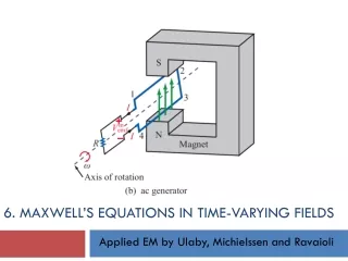
10. Time-Varying Fields Faraday’s Law continued According to Faraday’s law, a time-varying magnetic flux through a loop of wire results in a voltage across the loop terminals: The negative sign shows that the induced voltage acts in such a way as to oppose the change of flux producing it (Lenz’s law). Induced magnetic field (when circuit is closed) Increasing time-varying magnetic field Direction of the integration path I 3 2 - R + 1 4 The terminals are far away from the time-varying magnetic field If N-turn coil instead of single loop Consider now terminals 3 and 4, and 1 and 2 A time-varying magnetic flux through a loop wire results in the appearance of a voltage across its terminals. 2 3 No contribution from 2-3 and 4-1 because the wire is a perfect conductor 1 4 Integration path

11. Time-Varying Fields Faraday’s Law continued Example: An N-turn coil having an area A rotates in a uniform magnetic field The speed of rotation is n revolutions per second. Find the voltage at the coil terminals. rad Rotation Shaft

12. Time-Varying Fields Faraday’s Law continued Boundary Condition on Tangential Electric Field Using Faraday’s law, , we can obtain boundary condition on the tangential component of at a dielectric boundary. Medium 1 Medium 2 (unless ) L 3 L 1 - continuous at the boundary (For the normal component: ) at a dielectric boundary

13. Time-Varying Fields Inductance A circuit carrying current I produces a magnetic field which causes a flux to pass through each turn of the circuit. If the medium surrounding the circuit is linear, the flux is proportional to the current I producing it . For a time-varying current, according to Faraday’s law, we have - + (voltage induced across coil) I I , H (henry) Magnetic field B produced by a circuit. Self-inductanceL is defined as the ratio of the magnetic flux linkage to the current I.

14. Time-Varying Fields Inductance continued In an inductor such as a coaxial or a parallel-wire transmission line, the inductance produced by the flux internal to the conductor is called the internal inductance Lin while that produced by the flux external to it is called external inductance ( ) Let us find of a very long rectangular loop of wire for which , and . This geometry represents a parallel-conductor transmission line. Transmission lines are usually characterized by per unit length parameters. Wire radius = a 1 w I S h Finding the inductance per unit length of a parallel-conductor transmission line.

15. Time-Varying Fields Inductance continued The magnetic field produced by each of the long sides of the loop is given approximately by Parallel – conductor transmission line , H/m (per unit length) The internal inductance for nonferromagnetic materials is usually negligible compared to . Let us find the inductance per unit length of a coaxial transmission line. We assume that the currents flow on the surface of the conductors, which have no resistance. h b a I z Finding the inductance per unit length of a coaxial transmission line.

16. Time-Varying Fields Inductance continued Resistance Since R=0, has only radial component and therefore the segments 3 and 4 contribute nothing to the line integral. H/m (from previous work)

17. Time-Varying Fields General Forms of Maxwell’s Equations DifferentialIntegralRemarks 1 Gauss’ Law Nonexistence of isolated magnetic charge 2 Faraday’s Law 3 4 Ampere’s circuital law In 1 and 2, S is a closed surface enclosing the volume V In 2 and 3, L is a closed path that bounds the surface S

18. Time-Varying Fields Electric fields can originate on positive charges and can end on negative charges. But since nature has neglected to supply us with magnetic charges, magnetic fields cannot begin or end; they can only form closed loops.

19. Time-Varying Fields Sinusoidal Fields In electromagnetics, information is usually transmitted by imposing amplitude, frequency, or phase modulation on a sinusoidal carrier. Sinusoidal (or time-harmonic) analysis can be extended to most waveforms by Fourier and Laplace transform techniques. Sinusoids are easily expressed in phasors, which are more convenient to work with. Let us consider the “curl H” equation. Its phasor representation is is a vector function of position, but it is independent of time. The three scalar components of are complex numbers; that is, if then

20. Time-Varying Fields Sinusoidal Fields continued Time-Harmonic Maxwell’s Equations Assuming Time Factor . Point FormIntegral Form

21. Time-Varying Fields Maxwell’s Equations continued Electrostatics Electrodynamics (a) Magnetostatics (c) Free magnetic charge density ( ) (b) Electromagnetic flow diagram showing the relationship between the potentials and vector fields: (a) electrostatic system, (b) magnetostatic system, (c) electromagnetic system. [Adapted with permission from IEE Publishing Department]

22. Time-Varying Fields 0 z Skin depth x y The Skin Effect When time-varying fields are present in a material that has high conductivity, the fields and currents tend to be confined to a region near the surface of the material. This is known as the “skin effect”. Skin effect increases the effective resistance of conductors at high frequencies. Let us consider the vector wave equation (Helmholtz’s equation) for the electric field: If the material in question is a very good conductor, so that , we can write Since we also have Consider current flowing in the +x direction through a conductive material filling the half-space z<0. The current density is independent of y and x, so that we have Current density at surface J0 (Air) Z>0 (Metal) Z<0 Magnitude of current density decreases exponentially with depth

23. Time-Varying Fields The Skin Effect continued As , the first term increases and would give rise to infinitely large currents. Since this is physically unreasonable, the constant A must vanish. From the condition when z=0 we have Current density magnitude decreases exponentially with depth. Its phase changes as well. and At 10mm 1mm At 0.1mm Skin depth versus frequency for copper

24. Time-Varying Fields The Skin Effect continued Skin Depth and Surface Resistance for Metals

25. Time-Varying Fields Time-Varying Fields Surface Impedance If , the total current per unit width is 45° out of phase with Jo Since we can write Voltage per unit length Surface impedance or Direction of current flow “ohms per square” w l If l=w (a square surface) Illustrating the concept of “ohms per square”

26. Time-Varying Fields Surface Impedance continued RSis equivalent to the dc resistance per unit length of the conductor having cross-sectional area Copper For a wire of radius a,

27. Time-Varying Fields Time-Varying Fields Surface Impedance continued Wire (copper) bond Plated metal connections z=? Substrate (a) Thickness of current layer = 0.6 μm = δ w x 100 μm 2 r δ= 0.6 μm 100 μm (Internal inductance) (b) (c) Finding the resistance and internal inductance of a wire bond. The bond, a length of wire connecting two pads on an IC, is shown in (a). (b) is a cross-sectional view showing skin depth. In (c) we imagine the conducting layer unfolded into a plane.