Download
1 / 16
180 likes | 611 Views
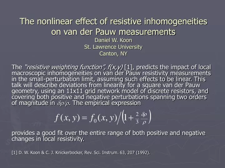
The nonlinear effect of resistive inhomogeneities on van der Pauw measurements Daniel W. Koon St. Lawrence University Canton, NY.

E N D
The nonlinear effect of resistive inhomogeneitieson van der Pauw measurementsDaniel W. KoonSt. Lawrence UniversityCanton, NY The “resistive weighting function”, f(x,y) [1], predicts the impact of local macroscopic inhomogeneities on van der Pauw resistivity measurements in the small-perturbation limit, assuming such effects to be linear. This talk will describe deviations from linearity for a square van der Pauw geometry, using an 11x11 grid network model of discrete resistors, and covering both positive and negative perturbations spanning two orders of magnitude in dr/r. The empirical expression provides a good fit over the entire range of both positive and negative changes in local resistivity. [1] D. W. Koon & C. J. Knickerbocker, Rev. Sci. Instrum. 63, 207 (1992).
Outline • Background • Model • A table-top, “analog computational” model of the square van der Pauw geometry. • Experimental results • Conclusions
The van der Pauw technique for resistivity measurement • Allows for resistivity measurement from arbitrary geometry with arbitrary placement of current and voltage leads. • Requires two independent resistance measurements (see figures above), but is often conducted using a single measurement. • Sample thickness is the only relevant geometrical factor (not shape or lateral dimensions). • But assumes uniform sample thickness & resistivity.
The resistive weighting function In general, the resistivity is not uniform, and so the measured resistivity, rm , is a weighted average of the local values of resistivity, r(x,y): where f (x,y) is the “resistive weighting function”, a measure of the impact that a local inhomogeneity has on the measured resistivity.
Results for the square vdP geometry The resistive weighting function, f (x,y), for (a) single resistance measurement, (b) resistance measurement averaged over two independent readings. D. W. Koon & C. J. Knickerbocker, Rev. Sci. Instrum. 63 (1), 207 (1992).
Results for other vdP geometries: The resistive weighting function, f (x,y), averaged over two independent readings, for (a) cross, (b) cloverleaf. D. W. Koon & C. J. Knickerbocker, Rev. Sci. Instrum. 67 (12), 4282 (1996).
Systems studied • Resistive weighting function • Square with electrodes at either edges or sides • Circular disc • Cross • Cloverleaf • Bar • 4-point probe arrays (both linear and square) • Hall weighting function (same geometries) • Finite-thickness effects • Experimental verification of both resistivity & Hall effect But, until now, no study of effect of large inhomogeneity.
Why should the effect of inhomogeneities be nonlinear? For a material of non-uniform resistivity, Locally tweaking the resistivity is equivalent to placing a dipole at that point which is parallel to and proportional to the local E-field. Since the perturbation alters the local E-field, -F, we would expect this to be a nonlinear effect. D. W. Koon & C. J. Knickerbocker, Rev. Sci. Instrum. 63 (1), 207 (1992).
“Analog computer” model: • Replace continuous 2D film with discrete individual resistors: • Edge resistors: R • Interior resistors: R/2 • Experimental implementation: • 11x11 grid array, with R/2=10kW. (308 resistors, total)
Perturbation I:Decrease local resistivity(“short-like” impurities) • Range: • dr/r = -1 to 0 • ds/s = R/r = 0 to • = 0 to 1, where
Perturbation II:Increase local resistivity(“open-like” impurities) • Range: • dr/r = 0 to • ds/s = - 1 to 0 • = -1 to 0, where
Experimental results I:Weighting function in 1111 grid The resistive weighting function f (x,y) (a) for a single measurement (b) for an average over two measurements. (Experimental results: 11x11 grid)
Experimental results II:Nonlinearity of f(x,y) at center • Impact of “shorting out” the center of 11x11 grid on the measured resistance, Rm, of the entire grid.
Experimental results III:Nonlinearity of the weighting function Increasing r Decreasing r Fit curve (in white):
Conclusions • Large resistive inhomogeneities produce nonlinear effects. • Decreasing the local resistivity produces up to 3x the expected effect (compared to linear approximation). • Increasing the local resistivity produces less than the expected effect. • These results are independent of location and well predicted by the expression:
Inconclusions (what’s next) • Why this expression? • What about additive effects? (simultaneous perturbation at 2+ locations)