Download
1 / 14
190 likes | 492 Views
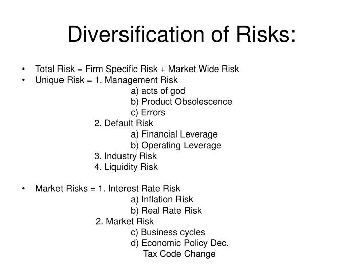
Diversification of Risks:. Total Risk = Firm Specific Risk + Market Wide Risk Unique Risk = 1. Management Risk a) acts of god b) Product Obsolescence c) Errors 2. Default Risk a) Financial Leverage b) Operating Leverage 3. Industry Risk 4. Liquidity Risk

E N D
Diversification of Risks: • Total Risk = Firm Specific Risk + Market Wide Risk • Unique Risk = 1. Management Risk a) acts of god b) Product Obsolescence c) Errors 2. Default Risk a) Financial Leverage b) Operating Leverage 3. Industry Risk 4. Liquidity Risk • Market Risks = 1. Interest Rate Risk a) Inflation Risk b) Real Rate Risk 2. Market Risk c) Business cycles d) Economic Policy Dec. Tax Code Change
Minimum Variance Portfolio • The maximum return any one will be willing to receive for a certain level of risk. • Adding the risk free modifies the efficient set to be linear now. Capital market line • Risk added by new asset is proportional to σim. Covariance is standardized by dividing it with σm². Beta = σim/ σm² and E(Ri)-Rf = β[E(Rm)-Rf]
Computing Beta: • Using regression: Ri = ά +βRm + εi σi² = β² σm² + σε² (The variation terms are related but not the standard deviation terms) Divide both sides by σ i²: 1=β² σm²/ σi²+ σε²/ σi² (proportion of market risk + proportion of unique risk) The relationship between coefficient of determination (R²) and correlation coefficient ρ. βi=Covariance(i,m)/var.(m)= σim/ σm²= ρim σiσm/σm² = Pim(σ i/ σ m) We know Ri²=β² σm²/ σi²= ρim²(σi²/ σm²)(σm²/σi²)= ρim² Ri = ρim
Two Basic ideas About Risk and ReturnMarket Model/Single Factor Model • CAPM: Ri=Rf+β(Rm-Rf) 1. Investors require compensation for risk 2. They care only about a stock’s contribution to portfolio. • Capital Asset Pricing Model: Example If Treasury bill rate = 5.6% Bristol Myers Squibb beta = .81 Expected market risk premium = 8.4% Ri=Rf+ β(Rm-Rf) =5.6+.81(8.4)=12.4% β=1 Ri=Rm β=0 Ri=Rf β>1 Ri>Rm β<1 Ri<Rm
Testing the Capital Asset Pricing Model • If a portfolio is efficient, there must be a straight line relationship between the expected return of any share and its beta relative to that portfolio. So testing whether the market portfolio is efficient. • Problems of testing: 1. measuring expected returns 2. measuring the market portfolio 3. measuring beta
Black, Jensen and Scholes’s Test of CAPM Theoretical line Average Monthly return Fitted line rm rf Beta Validity of Capital Asset Pricing Model Evidence is mixed 1. Long-run average returns are significantly related to beta 2. But beta is not a complete explanation. Low beta stocks have earned higher rates of return than predicted by the model. So have small company stocks.
CAPM • Capital Asset Pricing Model is AttractiveBecause: 1. It is simple and usually gives sensible answers. 2. It distinguishes between diversifiable and non-diversifiable risk. • Testing of CAPM is Controversial 1. No one knows for sure how to define and measure the market portfolio – and using the wrong index could lead to the wrong answer. 2. The model is hard to prove or disprove 3. The model has competitors e.g: arbitrage Pricing Model. Note: you can reject CAPM without rejecting the main points of modern portfolio theory.
The standard CAPM concentrates on how stocks contribute to the level and uncertainty of investor’s wealth. Consumption is outside the model. STOCKS (And Other Risky Assets) Standard CAPM assumes investors are Concerned with the amount and uncertainty of future wealth Market risk Makes wealth Uncertain. WEALTH = MARKET PORTFOLIO
The consumption CAPM defines risk as a stock’s contribution to uncertainty about consumption. Wealth (the intermediate step between stock returns and consumption) drops out of the model. STOCKS (And Other Risky Assets) Wealth is uncertain. Consumption CAPM connects uncertainty about stock returns directly to uncertainty about consumption. WEALTH Consumption is uncertain Consumption
Arbitrage pricing theory (APT) • Suppose returns depend on more than one factor i.e many factors: Return = a+b1(rfactor – rf)+b2(rfactor-rf)+…..+diversifiable noise A diversified portfolio that is not exposed to any factors must offer the risk-free rate: Return = a=rf when all b’s=0 But in general expected return depends on factor exposure Return – rf+b1(rfactor-rf)+b2(rfactor-rf)+… Where rfactor +expected return on “pure play” portfolio exposed only to factor i.
Arbitrage pricing Theory (APT) • Preserves distinction between diversifiable and non-diversifiable risk. • CAPM and APT can both hold-e.g. CAPM implies one factor APT, with rfactor + rm • But APT is more general – e.g. unlike CAPM, market portfolio doesn’t have to be efficient. • But usefulness of APT requires heavy-duty statistics to Identify factors Measure factor returns
Arbitrage Pricing Theory: Three ways to construct Factors: 1. Factor Analysis (FA) 2. Macro Economic Variables (MC) 3. Firm Characteristics (FC) Factor Analysis (FA): Developed using a statistical procedure called Factor Analysis ADVANTAGE: Best estimate of Factor DISADVANTAGE: No economic intuition Macro Economic Variables (MC): Use macro variables as factors e.g. productivity, Interest rates, inflation rates ADVANTAGE: Best economic interpretation DISADVANTAGE: Difficult to measure unanticipated changes. Firm Characteristics (FC): Use micro variables for firm as factors e.g. size, P/E, Book to market, etc. ADVANTAGE: More intuitive than FA DISADVANTAGE: Historical data? Future changes?
Chen, Roll and Ross (1986) The economic factors: 3. Industrial production : Survey of current 4. Consumption : Business 3. Oil prices : B of Labor Stats. 4. Inflation : Consumer Price Index 5. Treasury Bill Rate : 1 month T. bill 6. Long term Govt. Bonds :Treasury Bonds 10/15/20 yrs. 7. Low Grade Bonds : Baa or Lower 8. Equally Weighted Equities : NYSE 9. Value Weighted Equities : NYSE
Derived Series in Chen, Roll and Ross (1986): The variables used are: μP(t), γP(t) + Monthly or Annual Growth rate of industrial prod. E(I(t)) = expected Inflation UI(t) = unexpected Inflation RHO(t) = Real Int. Rate = Tb(t-1)-I(t) DEI(t) = Change in expected inflation E[I(t+1)]-E[I(t/t-1] URP(t) = Risk Premium Baa(t)-LGB(t) UTS(t) = Term structure LGB(t)-TB(t-1) Regression Reformed: R=a+βMP*MP+βDEI*DEI+βURP*URP+βUTS*UTS+Rm+Σj