Chap 2. The Geometry of LP

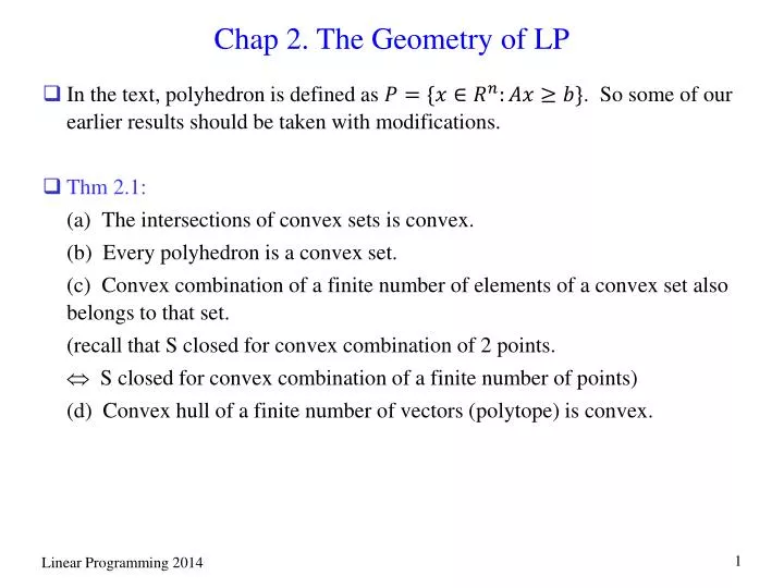
1. Chap 2. The Geometry of LP • In the text, polyhedron is defined as . So some of our earlier results should be taken with modifications. • Thm 2.1: (a) The intersections of convex sets is convex. (b) Every polyhedron is a convex set. (c) Convex combination of a finite number of elements of a convex set also belongs to that set. (recall that S closed for convex combination of 2 points.  S closed for convex combination of a finite number of points) (d) Convex hull of a finite number of vectors (polytope) is convex.

2. Pf) (a) Let , convex   , since convex   is convex. (b) Halfspace is convex. Polyhedron is intersection of halfspaces  From (a), P is convex. ( or we may directly show .) (c) Use induction. True for by definition. Suppose statement holds for elements. Suppose . Then and sum up to 1, hence  (d) Let be the convex hull of vectors and  for some . and sum up to 1  convex combination of  . 

3. Extreme points, vertices, and b.f.s’s • Def: (a) Extreme point ( as we defined earlier) (b) is a vertex if such that and . ( is a unique optimal solution of min ) (c) Consider polyhedron and . Then is a basic solution if all equality constraints are active at and linearly independent active constraints among the constraints active at . ( basic feasible solution if is basic solution and ) • Note: Earlier, we defined the extreme point same as in the text. Vertex as 0-dimensional face ( dim() + rank ) which is the same as the basic feasible solution defined in the text. We defined basic solution (and b.f.s) only for the standard LP. ( Definition (b) is new. It gives an equivalent characterization of extreme point. (b) can be extended to characterize a face of .

4. Fig. 2.6: Three constraints active at A, B, C, D. Only two constraints active at E. Note that D is not a basic solution since it does not satisfy the equality constraint. However, if is given as , D is a basic solution by the definition in the text, i.e. whether a solution is basic depends on the representation of . A C P E D B

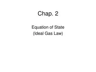
5. Fig. 2.7: A, B, C, D, E, F are all basic solutions. C, D, E, F are basic feasible solutions. A E D P F B C

6. Comparison of definitions in the notes and the text

7. Thm 2.3:, then vertex, extreme point, and b.f.s. are equivalent statements. Pf)We follow the definitions given in the text. We already showed in the notes that extreme point and 0-dimensional face ( , rank , b.f.s. in the text) are equivalent. To show all are equivalent, take the following steps: vertex (1)  extreme point (2)  b.f.s. (3)  vertex (1) vertex  extreme point Suppose is vertex, i.e. such that is unique minimum of min . If , then and . Hence  . Hence cannot be expressed as convex combination of two other points in .  extreme point.

8. (continued) (2) extreme point  b.f.s. Suppose is not a b.f.s.. Let . Since is not a b.f.s., the number of linearly independent vectors in . Hence nonzero such that . Consider . But, for sufficiently small positive , and , which implies is not an extreme point. (3) b.f.s.  vertex Let be a b.f.s. and let . Let . Then . , we have , hence optimal. For uniqueness, equality holds  . Since is a b.f.s., it is the unique solution of . Hence is a vertex. 

9. Note: Whether is a basic solution depends on the representation of . However, is b.f.s. if and only if extreme point and being extreme point is independent of the representation of . Hence the property of being a b.f.s. is also independent of the representation of . • Cor 2.1: For polyhedron , there can be finite number of basic or basic feasible solutions. • Def: Two distinct basic solutions are said to be adjacent if we can find linearly independent constraints that are active at both of them. ( In Fig 2.7, D and E are adjacent to B; A and C are adjacent to D.) If two adjacent basic solutions are also feasible, then the line segment that joins them is called an edge of the feasible set (one dimensional face).

10. 2.3 Polyhedra in standard form • Thm 2.4:, , full row rank. Then is a basic solution  satisfies and indices such that are linearly independent and . Pf) see text. ( To find a basic solution, choose linearly independent columns . Set for all , then solve for . ) • Def: basic variable, nonbasic variable, basis, basic columns, basis matrix . (see text) (  )

11. Def: For standard form problems, we say that two bases are adjacent if they share all but one basic column. • Note: A basis uniquely determines a basic solution. Hence if have two different basic solutions  have different bases. But two different bases may correspond to the same basic solution. (e.g. when ) Similarly, two adjacent basic solutions  two adjacent bases Two adjacent bases with different basic solutions  two adjacent basic solutions. However, two adjacent bases only not necessarily imply two adjacent basic solutions. The two solutions may be the same solution.

12. Check that full row rank assumption on results in no loss of generality. • Thm 2.5:, , rank is . , with linearly independent rows. Then . Pf) Suppose first rows of are linearly independent. is clear. Show . Every row of can be expressed as . Hence, for , , i.e. is also linear combination of . Suppose , then , Hence,  

13. 2.4 Degeneracy • Def 2.10: A basic solution is said to be degenerate if more than of the constraints are active at . • Def 2.11:, , full row rank. Then is a degenerate basic solution if more than of the components of are 0 ( i.e. some basic variables have 0 value) • For standard LP, if we have more than variables at 0 for a basic feasible solution , it means that more than of the nonnegativity constraints are active at in addition to the constraints in . The solution can be identified by defining nonbasic variables (value ). Hence, depending on the choice of nonbasic variables, we have different bases, but the solution is the same.

14. Fig 2.9: A and C are degenerate basic feasible solutions. B and E are nondegenerate. D is a degenerate basic solution. A D C P B E

15. Fig 2.11:-dimensional illustration of degeneracy. Here, , . A is nondegenerate and basic variables are . B is degenerate. We can choose as the nonbasic variables. Other possibilities are to choose , or to choose . A B

16. Degeneracy is not purely geometric property, it may depend on representation of the polyhedrom ex), We know that , but representation is different. Suppose is a nondegenerate basic feasible solution of . Then exactly of the variables are equal to 0. For , at the basic feasible solution , we have variables set to 0 and additional constraints are satisfied with equality. Hence, we have active constraints and is degenerate.

17. 2.5 Existence of extreme points • Def 2.12: Polyhedron contains a line if a vector and a nonzero such that for all . Note that if is a line in , then for all  Hence is a vector in the lineality space . (in ) • Thm 2.6:, then the following are equivalent. (a) has at least one extreme point. (b) does not contain a line. (c) vectors out of , which are linearly independent. Pf) see proof in the text.

18. Note that the conditions given in Thm 2.6 means that the lineality space . • Cor 2.2: Every nonempty bounded polyhedron (polytope) and every nonempty polyhedron in standard form has at least one basic feasible solution (extreme point).

19. 2.6 Optimality of extreme points • Thm 2.7: Consider the LP of minimizing over a polyhedron . Suppose has at least one extreme point and there exists an optimal solution. Then there exists an optimal solution which is an extreme point of . Pf) see text. • Thm 2.8: Consider the LP of minimizing over a polyhedron . Suppose has at least one extreme point. Then, either the optimal cost is , or there exists an extreme point which is optimal.

20. (continued) Idea of proof in the text) Consider any . Let Then we move to , where and . Then either the optimal cost is ( if the half line is in and ) or we meet a new inequality which becomes active ( cost does not increase). By repeating the process, we eventually arrive at an extreme point which has value not inferior to . Therefore, for any in , there exists an extreme point such that . Then we choose the extreme point which gives the smallest objective value with respect to .

21. ( alternative proof of Thm 2.8) . Pointedness of implies . Hence  , where are extreme rays of and are extreme points of and . Suppose such that , then LP is unbounded. ( For , for . Then  as ) Otherwise, for all , take such that . Then , . Hence LP is either unbounded or an extreme point of which is an optimal solution. Proof here shows that the existence of an extreme ray of the pointed recession cone ( if have min problem and polyhedron is ) such that is the necessary and sufficient condition for unboundedness of the LP. ( If has at least one extreme point, then LP is unbounded  an extreme ray in recession cone such that ) 